Understanding the Bellman Equation in Q-Learning

Notebook de Jupyter, 4 min de lectura.qlearning/bellman_equation.ipynb

En esta página

What is the Bellman Equation?
A Step-by-Step Example
Initial Q-Table
Step 1: Agent moves from S0 to S1
Step 2: Agent moves from S1 to S2 (The Goal!)
Step 3: A New Episode - Agent moves from S0 to S1 again
How it Looks in Code
Conclusion

This notebook breaks down the core of Q-Learning: the Bellman Equation. We'll go step-by-step to see how an agent's "brain"—the Q-table—is updated. We'll use a simple example inspired by the FrozenLake environment.

What is the Bellman Equation?

The Bellman Equation is the update rule used in Q-learning. It tells us how to improve our estimate for the value of a state-action pair based on new information we gather from the environment.

Here is the formula:

$Q(s, a) \leftarrow Q(s, a) + \alpha \left[ r + \gamma \max_{a'} Q(s', a') - Q(s, a) \right]$

It looks complex, but let's break it down into plain English:

New Q-value = Old Q-value + Learning Rate * (Temporal Difference Error)

Where:

Q(s, a): The current Q-value for being in state s and taking action a. This is our old estimate.
α (alpha): The Learning Rate (e.g., 0.1). This controls how much we update our Q-value. A small α means we learn slowly, while a large α means we learn fast.
r: The immediate Reward we get after taking action a from state s.
γ (gamma): The Discount Factor (e.g., 0.95). This determines how much we value future rewards. A γ close to 1 means we care a lot about future rewards, while a γ close to 0 means we only care about the immediate reward.
max Q(s', a'): The best possible Q-value we can get from our next state s'. This is the agent looking one step ahead and picking the most valuable action from its new position.
r + γ * max Q(s', a'): This is the learned value or the "new, better estimate" of the Q-value. It's the immediate reward plus the discounted estimate of the future reward.
[...] - Q(s, a): This whole part is the Temporal Difference (TD) Error. It's the difference between our new estimate and our old one. It represents the "surprise" or how wrong our initial estimate was.

A Step-by-Step Example

Let's simulate a tiny piece of the FrozenLake world. Imagine this simple 3-state environment:

Start (S0) <-> Frozen (S1) <-> Goal (S2)

import gymnasium as gym
import matplotlib.pyplot as plt

env = gym.make('FrozenLake-v1', desc=["SFG"], is_slippery=False, render_mode="rgb_array")
env.reset()

def show_env(env):
    '''Render and display the environment in the notebook.'''
    img = env.render()
    plt.imshow(img)
    plt.axis('off')
    plt.show()

show_env(env)

/media/NOCTURNOEXTRA/Alejandro/wip-clase/.venv/lib/python3.13/site-packages/pygame/pkgdata.py:25: UserWarning: pkg_resources is deprecated as an API. See https://setuptools.pypa.io/en/latest/pkg_resources.html. The pkg_resources package is slated for removal as early as 2025-11-30. Refrain from using this package or pin to Setuptools<81.
  from pkg_resources import resource_stream, resource_exists

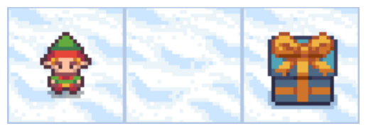
States: S0, S1, S2
Actions: 0 (Left), 1 (Right)
Rewards:
- +1 for reaching the Goal (S2)
- 0 for any other move.

Let's set our hyperparameters:

Learning Rate (α) = 0.1
Discount Factor (γ) = 0.9

Initial Q-Table

Our agent starts with no knowledge. The Q-table is a [states x actions] matrix filled with zeros.

\begin{array}{c c} & \color{gray} \begin{matrix} \text{Left (0)} & \text{Right (1)} \end{matrix} \\ \color{gray} \begin{matrix} \text{S0} \\ \text{S1} \\ \text{S2} \end{matrix} & \begin{bmatrix} 0 & \quad 0 \\ 0 & \quad 0 \\ 0 & \quad 0 \end{bmatrix} \end{array}

import numpy as np

q_table = np.zeros((3, 2)) # 3 states, 2 actions

print("Initial Q-Table:")
print(q_table)

Initial Q-Table:
[[0. 0.]
 [0. 0.]
 [0. 0.]]

Step 1: Agent moves from S0 to S1

Current State (s): S0
Action (a): 1 (Move Right)
Observation:
- New State (s') = S1
- Reward (r) = 0

Now, let's plug this into the Bellman equation to update Q(S0, Right).

Formula: Q(s, a) = Q(s, a) + α * [r + γ * max Q(s', a') - Q(s, a)]

Calculation:

Q(S0, Right) = q_table[0, 1] = 0
α = 0.1
r = 0
γ = 0.9
max Q(S1, a'): The best Q-value from state S1. We look at the row for S1 in our Q-table (q_table[1]). The values are [0, 0]. The max value is 0.

Let's substitute: New Q(S0, Right) = 0 + 0.1 * [0 + 0.9 * 0 - 0] New Q(S0, Right) = 0

Not very exciting. The Q-value didn't change because no reward was found. This is common at the beginning of training.

Step 2: Agent moves from S1 to S2 (The Goal!)

Current State (s): S1
Action (a): 1 (Move Right)
Observation:
- New State (s') = S2 (Goal)
- Reward (r) = +1

Let's update Q(S1, Right).

Calculation:

Q(S1, Right) = q_table[1, 1] = 0
α = 0.1
r = 1
γ = 0.9
max Q(S2, a'): The best Q-value from state S2. The S2 row in our Q-table (q_table[2]) is [0, 0]. The max value is 0. (S2 is a terminal state, so future rewards from here are 0).

Let's substitute: New Q(S1, Right) = 0 + 0.1 * [1 + 0.9 * 0 - 0] New Q(S1, Right) = 0.1 * [1] New Q(S1, Right) = 0.1

This is our first update! The agent learned that moving right from S1 is slightly good.

q_table[1, 1] = 0.1
print("Q-Table after Step 2:")
print(q_table)

Q-Table after Step 2:
[[0.  0. ]
 [0.  0.1]
 [0.  0. ]]

Step 3: A New Episode - Agent moves from S0 to S1 again

Now the magic happens. The reward information starts to flow backward.

Current State (s): S0
Action (a): 1 (Move Right)
Observation:
- New State (s') = S1
- Reward (r) = 0

Let's update Q(S0, Right) again.

Calculation:

Q(S0, Right) = q_table[0, 1] = 0 (from before)
α = 0.1
r = 0
γ = 0.9
max Q(S1, a'): This is the key difference! We look at the row for S1 in our updated Q-table (q_table[1]). The values are [0, 0.1]. The max value is now 0.1.

Let's substitute: New Q(S0, Right) = 0 + 0.1 * [0 + 0.9 * 0.1 - 0] New Q(S0, Right) = 0.1 * [0.09] New Q(S0, Right) = 0.009

The value of being at S0 and moving right has now increased! The agent is learning that this action leads to a state (S1) which has a known, positive future value. The reward from reaching the goal is slowly propagating backward to the states that lead to it.

q_table[0, 1] = 0.009
print("Q-Table after Step 3:")
print(q_table)

Q-Table after Step 3:
[[0.    0.009]
 [0.    0.1  ]
 [0.    0.   ]]

How it Looks in Code

Here is the Python code from the frozen_lake.ipynb notebook that implements this exact formula. You can see how each variable maps directly to the equation.

# From the training loop:
# Qtable[state][action] = Qtable[state][action] + learning_rate * (
#     reward + gamma * np.max(Qtable[new_state]) - Qtable[state][action]
# )

# Let's map it to our last calculation:
s = 0
a = 1
s_prime = 1
r = 0

learning_rate = 0.1
gamma = 0.9

# q_table before update
q_table_before = np.array([[0., 0.], [0., 0.1], [0., 0.]])

# The Bellman update in code
old_q_value = q_table_before[s, a]                 # Q(s, a)
max_future_q = np.max(q_table_before[s_prime])   # max Q(s', a')
td_error = r + gamma * max_future_q - old_q_value

new_q_value = old_q_value + learning_rate * td_error

print(f"Old Q-value: {old_q_value}")
print(f"Max future Q-value from S{s_prime}: {max_future_q}")
print(f"TD Error: {td_error:.3f}")
print(f"New Q-value for Q(S{s}, Right): {new_q_value:.3f}")

Old Q-value: 0.0
Max future Q-value from S1: 0.1
TD Error: 0.090
New Q-value for Q(S0, Right): 0.009

Conclusion

By repeatedly applying the Bellman Equation over thousands of episodes, the agent explores the environment and slowly builds a Q-table that accurately predicts the long-term reward of every action from every state. The initial small reward values gradually spread and flow backward from the goal state, carving out an optimal path.

The final Q-table in frozen_lake.ipynb is simply the result of this process happening thousands of times, creating a complete "cheat sheet" for navigating the icy terrain.