Random Forests: Ensemble Learning

Introduction to Random Forests

As we saw earlier, decision trees have a major limitation: they tend to overfit the training data, especially when allowed to grow deep. A single decision tree has high variance - small changes in the training data can result in very different tree structures.

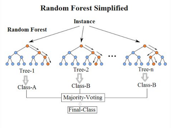
Random Forests solve this problem using an ensemble learning technique. Instead of relying on a single decision tree, Random Forests build many trees and combine their predictions. This is based on the principle that "the wisdom of the crowd" is often more accurate than any individual.

Key idea: Train multiple decision trees on different random subsets of the data and features, then aggregate their predictions:

Classification: Use majority voting (the class that receives the most votes)
Regression: Average the predictions of all trees

This approach dramatically reduces overfitting while maintaining the interpretability benefits of decision trees.

How Random Forests Work

Random Forests use two key sources of randomness to create diverse trees:

Bootstrap Aggregating (Bagging):
- Each tree is trained on a random sample of the training data (with replacement)
- This is called bootstrap sampling
- Typically, each sample contains about 63% of the original data
Random Feature Selection:
- At each split in a tree, only a random subset of features is considered
- This ensures trees are different from each other
- Typical values: $\sqrt{n_{features}}$ for classification, $n_{features}/3$ for regression

Algorithm steps:

Create N bootstrap samples from the training data
For each sample, train a decision tree:
- At each node, select a random subset of features
- Choose the best split from this subset
To make a prediction:
- Classification: Each tree votes, majority wins
- Regression: Average all tree predictions

Random Forest Illustration

Random Forest for Classification

from sklearn.ensemble import RandomForestClassifier
from sklearn.model_selection import train_test_split
from sklearn.metrics import accuracy_score, classification_report

# Using the iris dataset
from sklearn.datasets import load_iris
iris = load_iris()
X = iris.data
y = iris.target

# Split data into training and test sets
X_train, X_test, y_train, y_test = train_test_split(X, y, test_size=0.3, random_state=42)

# Train a single decision tree
single_tree = DecisionTreeClassifier(random_state=42).fit(X_train, y_train)

# Train a Random Forest with 100 trees
rf_classifier = RandomForestClassifier(n_estimators=100, random_state=42).fit(X_train, y_train)

# Compare predictions
tree_pred = single_tree.predict(X_test)
rf_pred = rf_classifier.predict(X_test)

print("Single Decision Tree Accuracy:", accuracy_score(y_test, tree_pred))
print("Random Forest Accuracy:", accuracy_score(y_test, rf_pred))
print("\nRandom Forest Classification Report:")
print(classification_report(y_test, rf_pred, target_names=iris.target_names))

Single Decision Tree Accuracy: 1.0
Random Forest Accuracy: 1.0

Random Forest Classification Report:
              precision    recall  f1-score   support

      setosa       1.00      1.00      1.00        19
  versicolor       1.00      1.00      1.00        13
   virginica       1.00      1.00      1.00        13

    accuracy                           1.00        45
   macro avg       1.00      1.00      1.00        45
weighted avg       1.00      1.00      1.00        45

Random Forest for Regression

Let's compare a single regression tree with a Random Forest on the salary dataset:

from sklearn.ensemble import RandomForestRegressor
from sklearn.metrics import mean_squared_error, r2_score

# Load salary data
df = pd.read_csv("data/salaries.csv")

# Train models
tree_reg_full = DecisionTreeRegressor(random_state=42).fit(df[["YearsExperience"]], df["Salary"])
rf_regressor = RandomForestRegressor(n_estimators=100, random_state=42).fit(df[["YearsExperience"]], df["Salary"])

# Create prediction points
x_plot = np.linspace(0, 12, 1000)
tree_predictions = tree_reg_full.predict(x_plot.reshape(-1, 1))
rf_predictions = rf_regressor.predict(x_plot.reshape(-1, 1))

# Visualize
plt.figure(figsize=(12, 5))

plt.subplot(1, 2, 1)
plt.scatter(df['YearsExperience'], df['Salary'], label='Actual data', alpha=0.7)
plt.plot(x_plot, tree_predictions, color='red', label='Single Decision Tree', linewidth=2)
plt.xlabel('Years of Experience')
plt.ylabel('Salary')
plt.title('Single Decision Tree (Overfitting)')
plt.legend()
plt.grid(True, alpha=0.3)

plt.subplot(1, 2, 2)
plt.scatter(df['YearsExperience'], df['Salary'], label='Actual data', alpha=0.7)
plt.plot(x_plot, rf_predictions, color='green', label='Random Forest', linewidth=2)
plt.xlabel('Years of Experience')
plt.ylabel('Salary')
plt.title('Random Forest (Smooth Prediction)')
plt.legend()
plt.grid(True, alpha=0.3)

plt.tight_layout()
plt.show()

# Compare metrics
train_pred_tree = tree_reg_full.predict(df[["YearsExperience"]])
train_pred_rf = rf_regressor.predict(df[["YearsExperience"]])

print(f"Single Tree - MSE: {mean_squared_error(df['Salary'], train_pred_tree):.2f}, R²: {r2_score(df['Salary'], train_pred_tree):.4f}")
print(f"Random Forest - MSE: {mean_squared_error(df['Salary'], train_pred_rf):.2f}, R²: {r2_score(df['Salary'], train_pred_rf):.4f}")

/home/avidaldo/TRABAJO/wip-clase/.venv/lib/python3.12/site-packages/sklearn/utils/validation.py:2749: UserWarning: X does not have valid feature names, but DecisionTreeRegressor was fitted with feature names
/home/avidaldo/TRABAJO/wip-clase/.venv/lib/python3.12/site-packages/sklearn/utils/validation.py:2749: UserWarning: X does not have valid feature names, but RandomForestRegressor was fitted with feature names

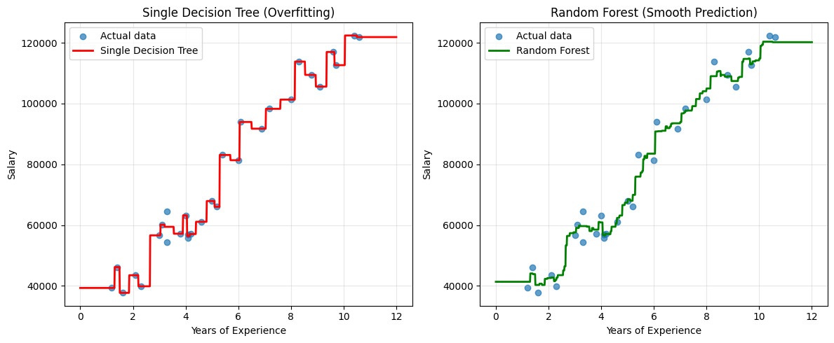
Single Tree - MSE: 1689209.48, R²: 0.9977
Random Forest - MSE: 6932913.11, R²: 0.9905

Notice how the Random Forest produces a much smoother prediction curve compared to the jagged overfitted curve of a single decision tree!

Feature Importance

One of the great advantages of Random Forests is that they can tell us which features are most important for making predictions. This is calculated by measuring how much each feature decreases the impurity (Gini or entropy) across all trees.

# Feature importance for the iris classification
import pandas as pd
import matplotlib.pyplot as plt

importances = rf_classifier.feature_importances_
feature_names = iris.feature_names

# Create a dataframe for better visualization
feature_importance_df = pd.DataFrame({
    'Feature': feature_names,
    'Importance': importances
}).sort_values('Importance', ascending=False)

print("Feature Importance:")
print(feature_importance_df)

# Visualize
plt.figure(figsize=(8, 5))
plt.barh(feature_importance_df['Feature'], feature_importance_df['Importance'])
plt.xlabel('Importance')
plt.title('Feature Importance in Random Forest')
plt.gca().invert_yaxis()
plt.tight_layout()
plt.show()

Feature Importance:
             Feature  Importance
3   petal width (cm)    0.433982
2  petal length (cm)    0.417308
0  sepal length (cm)    0.104105
1   sepal width (cm)    0.044605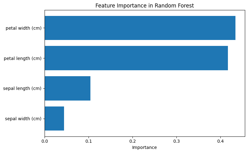

Important Hyperparameters

Random Forests have several hyperparameters that can be tuned:

Parameter	Description	Default	Impact
`n_estimators`	Number of trees in the forest	100	More trees = better performance but slower. Usually 100-500 is good
`max_depth`	Maximum depth of each tree	None (unlimited)	Controls overfitting. Lower values prevent overfitting
`min_samples_split`	Min samples required to split a node	2	Higher values prevent overfitting
`min_samples_leaf`	Min samples required in a leaf node	1	Higher values create smoother models
`max_features`	Max features to consider per split	'sqrt' (classification) '1.0' (regression)	Lower values increase diversity between trees
`random_state`	Seed for reproducibility	None	Set to a number for reproducible results
`n_jobs`	Number of CPU cores to use	None (1 core)	Set to -1 to use all available cores

Advantages and Disadvantages of Random Forests

Advantages:

Reduces overfitting: By averaging multiple trees, variance is reduced significantly
High accuracy: Often achieves excellent performance out-of-the-box
Handles missing data: Can maintain accuracy even with missing values
Works with both categorical and numerical features: Minimal preprocessing required
Feature importance: Provides insights into which features matter most
Robust to outliers: Individual trees may overfit outliers, but ensemble averages them out
Parallelizable: Trees can be trained independently on multiple CPU cores

Disadvantages:

Less interpretable: Cannot visualize hundreds of trees like a single tree
Slower prediction: Must aggregate predictions from many trees
Larger model size: Requires storing multiple trees in memory
Not ideal for extrapolation: Cannot predict beyond the range of training data
Can overfit noisy data: If trees are too deep and dataset is very noisy

Summary: Decision Trees vs. Random Forests

Aspect	Single Decision Tree	Random Forest
Model type	Single model	Ensemble of models
Overfitting	High tendency to overfit	Reduced overfitting
Variance	High variance	Low variance
Bias	Low bias (if deep)	Slightly higher bias
Interpretability	Highly interpretable	Less interpretable
Training time	Fast	Slower (trains multiple trees)
Prediction time	Very fast	Slower (aggregates predictions)
Accuracy	Lower (especially on test data)	Higher (more robust)
When to use	Need interpretability, small dataset	Need accuracy, can afford computation

Key Takeaway: Random Forests trade some interpretability and speed for significantly better generalization and accuracy. They are one of the most powerful and widely-used machine learning algorithms in practice.

Additional Resources on Random Forests

Random Forests - Scikit-learn Documentation
StatQuest: Random Forests Part 1 - Building, Using and Evaluating
StatQuest: Random Forests Part 2 - Missing Data and Clustering
Original paper: Breiman, L. (2001). "Random Forests". Machine Learning. 45 (1): 5–32.