XOR, Linear Separability, and Why Non-linearity Matters

Notebook de Jupyter, 5 min de lectura.pytorch/01-deep-learning-fundamentals/complementary/xor_linearity.ipynb

En esta página

The XOR idea
What does "linearly separable" mean?
Perceptron, linear regression, logistic regression
Demo: linear models fail on XOR
Feature engineering vs. representation learning
Why activations are the key ingredient
Non-linearity: a tiny MLP solves XOR
Universal Approximation Theorem
Hidden layer size experiment
What to take away

This notebook connects a few ideas that show up early in deep learning:

XOR as the smallest example of a feature interaction
What linearly separable means in practice
How perceptron, linear regression, and logistic regression are related
Why activation functions (non-linearity) are the key ingredient behind deep learning

We use minimal math and rely on plots + code.

Prerequisites: 01_intro_neural_networks.ipynb, 02_pytorch_basics.ipynb

The XOR idea

XOR means: either condition A or condition B is true, but not both.

x₁	x₂	XOR
0	0	0
0	1	1
1	0	1
1	1	0

Why do we care? Because XOR is the smallest example that requires combining conditions — the kind of logic that appears in real projects as feature interactions.

import numpy as np
import matplotlib.pyplot as plt

def make_noisy_xor(n_per_corner: int = 200, noise: float = 0.25, seed: int = 0):
    rng = np.random.default_rng(seed)
    corners = np.array([[-1, -1], [-1, 1], [1, -1], [1, 1]], dtype=np.float32)
    X = np.repeat(corners, repeats=n_per_corner, axis=0)
    X = X + rng.normal(0.0, noise, size=X.shape).astype(np.float32)
    y = ((X[:, 0] > 0) ^ (X[:, 1] > 0)).astype(np.float32)
    return X, y

X, y = make_noisy_xor()

plt.figure(figsize=(4, 4))
plt.scatter(X[y == 0, 0], X[y == 0, 1], s=12, alpha=0.7, label="class 0")
plt.scatter(X[y == 1, 0], X[y == 1, 1], s=12, alpha=0.7, label="class 1")
plt.title("XOR dataset (not linearly separable)")
plt.xlabel("x1")
plt.ylabel("x2")
plt.grid(True, alpha=0.2)
plt.legend(loc="upper right")
plt.show()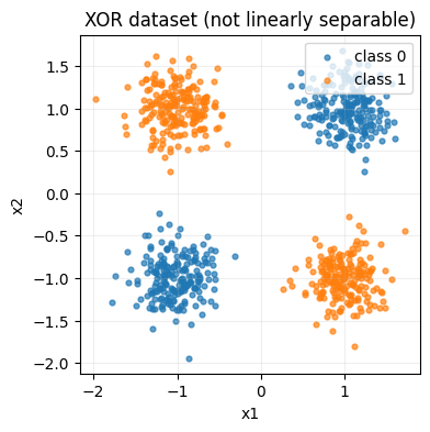

What does "linearly separable" mean?

A model is linear (for classification) if it can only separate classes using one straight boundary:

A line in 2D
A plane in 3D
A hyperplane in higher dimensions

If the data can't be split by one straight boundary, then no amount of training will make a purely linear model solve it — it's a representation limitation, not an optimization limitation.

Perceptron, linear regression, logistic regression

All three start with the same core computation — a linear score:

$\text{score} = w_1 x_1 + w_2 x_2 + \ldots + b$

They differ in what happens after and what loss they optimize:

Model	After the linear score	Loss	Use for
Linear regression	Nothing (raw number)	MSE	Regression
Perceptron (classic)	Hard threshold (step function)	Perceptron loss	Binary classification (historical)
Logistic regression	Smooth threshold (sigmoid)	BCE	Binary classification (modern baseline)

In PyTorch, a single nn.Linear(2, 1) + sigmoid + BCE loss is logistic regression.

Demo: linear models fail on XOR

import torch
import torch.nn as nn

torch.manual_seed(0)

X_t = torch.from_numpy(X)
y_t = torch.from_numpy(y).reshape(-1, 1)

def accuracy_from_logits(logits: torch.Tensor, y_true: torch.Tensor) -> float:
    preds = (torch.sigmoid(logits) > 0.5).to(dtype=y_true.dtype)
    return float((preds == y_true).to(torch.float32).mean().item())

def plot_probability_surface(ax, model: nn.Module, title: str):
    xx, yy = np.meshgrid(np.linspace(-2.5, 2.5, 250), np.linspace(-2.5, 2.5, 250))
    grid = torch.from_numpy(np.c_[xx.ravel(), yy.ravel()].astype(np.float32))
    with torch.no_grad():
        probs = torch.sigmoid(model(grid)).reshape(xx.shape).cpu().numpy()
    ax.contourf(xx, yy, probs, levels=25, alpha=0.65)
    ax.set_title(title)
    ax.set_xlabel("x1")
    ax.set_ylabel("x2")
    ax.grid(True, alpha=0.2)

def scatter_data(ax):
    ax.scatter(X[y == 0, 0], X[y == 0, 1], s=10, alpha=0.7, label="class 0")
    ax.scatter(X[y == 1, 0], X[y == 1, 1], s=10, alpha=0.7, label="class 1")
    ax.legend(loc="upper right")

# 1) Linear regression forced into classification (MSE + threshold)
linreg = nn.Linear(2, 1)
opt = torch.optim.SGD(linreg.parameters(), lr=0.1)
for _ in range(400):
    opt.zero_grad()
    loss = nn.MSELoss()(linreg(X_t), y_t)
    loss.backward()
    opt.step()

# 2) Logistic regression (BCEWithLogitsLoss)
logreg = nn.Linear(2, 1)
opt = torch.optim.SGD(logreg.parameters(), lr=0.5)
for _ in range(400):
    opt.zero_grad()
    loss = nn.BCEWithLogitsLoss()(logreg(X_t), y_t)
    loss.backward()
    opt.step()

with torch.no_grad():
    print(f"Linear regression accuracy: {accuracy_from_logits(linreg(X_t), y_t):.3f}")
    print(f"Logistic regression accuracy: {accuracy_from_logits(logreg(X_t), y_t):.3f}")

fig, axes = plt.subplots(1, 2, figsize=(9, 4))
plot_probability_surface(axes[0], linreg, "Linear regression (still linear)")
scatter_data(axes[0])
plot_probability_surface(axes[1], logreg, "Logistic regression (still linear)")
scatter_data(axes[1])
plt.tight_layout()
plt.show()

Linear regression accuracy: 0.500
Logistic regression accuracy: 0.500

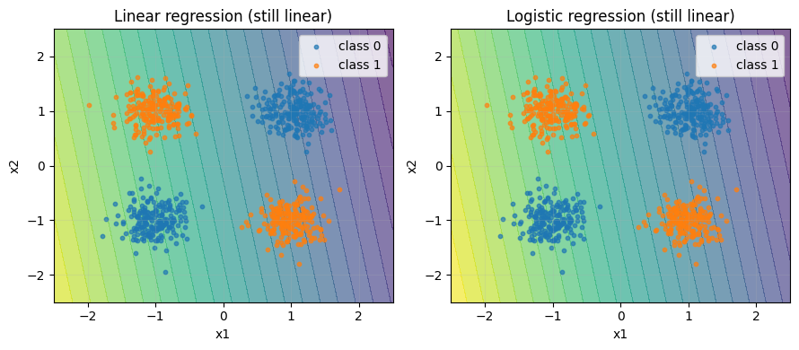
Both models are still linear in the inputs, so they share the same fundamental limitation on XOR. Logistic regression is a better classification tool, but it's still a linear classifier.

Feature engineering vs. representation learning

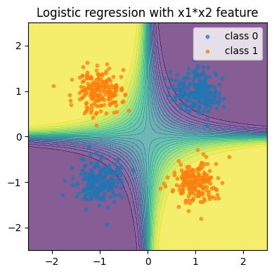
One way to solve XOR with a linear model is to manually add a feature interaction.

If you add x₃ = x₁ × x₂, the classes become easy to separate with a straight boundary in the expanded 3D space.

This is a key connection:

Classical ML: you hand-engineer interaction features (polynomial features, domain knowledge).
Deep learning: you let the network learn useful interactions automatically via hidden layers + activations.

# Add an interaction feature: x3 = x1 * x2
X3 = (X[:, 0] * X[:, 1]).reshape(-1, 1).astype(np.float32)
X_fe_t = torch.from_numpy(np.concatenate([X.astype(np.float32), X3], axis=1))

logreg_fe = nn.Linear(3, 1)
opt = torch.optim.SGD(logreg_fe.parameters(), lr=0.5)
for _ in range(400):
    opt.zero_grad()
    loss = nn.BCEWithLogitsLoss()(logreg_fe(X_fe_t), y_t)
    loss.backward()
    opt.step()

with torch.no_grad():
    print(f"Logistic regression + x1*x2 feature accuracy: {accuracy_from_logits(logreg_fe(X_fe_t), y_t):.3f}")

fig, ax = plt.subplots(figsize=(4, 4))
xx, yy = np.meshgrid(np.linspace(-2.5, 2.5, 250), np.linspace(-2.5, 2.5, 250))
grid_xy = np.c_[xx.ravel(), yy.ravel()].astype(np.float32)
grid_x3 = (grid_xy[:, 0] * grid_xy[:, 1]).reshape(-1, 1)
grid_fe = torch.from_numpy(np.concatenate([grid_xy, grid_x3], axis=1))
with torch.no_grad():
    probs = torch.sigmoid(logreg_fe(grid_fe)).reshape(xx.shape).cpu().numpy()
ax.contourf(xx, yy, probs, levels=25, alpha=0.65)
scatter_data(ax)
ax.set_title("Logistic regression with x1*x2 feature")
plt.tight_layout()
plt.show()

Logistic regression + x1*x2 feature accuracy: 1.000

Why activations are the key ingredient

A common misunderstanding: "if one linear layer isn't enough, let's stack two."

But linear → linear is still linear — the composition collapses into a single linear transformation. Stacking layers only becomes interesting once you insert non-linear activations (ReLU, tanh, …) between them.

# Proof: two stacked linear layers = one linear layer
torch.manual_seed(0)
layer1 = nn.Linear(2, 4)
layer2 = nn.Linear(4, 1)

x = torch.randn(10, 2)
y_stacked = layer2(layer1(x))

# Equivalent single linear layer
W_equiv = layer2.weight @ layer1.weight
b_equiv = layer2.bias + (layer2.weight @ layer1.bias)
y_equiv = x @ W_equiv.T + b_equiv

print(f"Max difference: {(y_stacked - y_equiv).abs().max().item():.6g}")

Max difference: 2.98023e-08

Non-linearity: a tiny MLP solves XOR

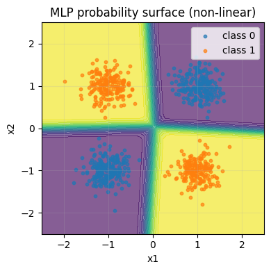
Instead of manually adding x₁ × x₂, we use a small network with an activation function. The hidden layer learns intermediate "detectors" that behave like engineered features — but learned from data.

mlp = nn.Sequential(nn.Linear(2, 8), nn.ReLU(), nn.Linear(8, 1))
opt = torch.optim.Adam(mlp.parameters(), lr=0.05)
bce = nn.BCEWithLogitsLoss()

for _ in range(600):
    opt.zero_grad()
    loss = bce(mlp(X_t), y_t)
    loss.backward()
    opt.step()

with torch.no_grad():
    print(f"MLP accuracy: {accuracy_from_logits(mlp(X_t), y_t):.3f}")

fig, ax = plt.subplots(figsize=(4, 4))
plot_probability_surface(ax, mlp, "MLP probability surface (non-linear)")
scatter_data(ax)
plt.tight_layout()
plt.show()

MLP accuracy: 1.000

Universal Approximation Theorem

A feedforward network with a single hidden layer containing enough neurons can approximate any continuous function on a compact subset of ℝⁿ.

Implications:

MLPs are theoretically powerful enough for any task.
"Enough" neurons may be impractically large.
Deeper networks often work better than wider ones in practice.
Finding the right weights is the hard part (training).

Hidden layer size experiment

hidden_sizes = [2, 4, 8, 16, 32]
results = {}

for h in hidden_sizes:
    mlp = nn.Sequential(nn.Linear(2, h), nn.ReLU(), nn.Linear(h, 1))
    opt = torch.optim.Adam(mlp.parameters(), lr=0.05)
    for _ in range(600):
        opt.zero_grad()
        bce(mlp(X_t), y_t).backward()
        opt.step()
    with torch.no_grad():
        results[h] = accuracy_from_logits(mlp(X_t), y_t)
    print(f"Hidden size {h:2d}: {results[h]:.3f}")

Hidden size  2: 0.999
Hidden size  4: 0.999
Hidden size  8: 1.000
Hidden size 16: 1.000
Hidden size 32: 1.000

Even 2 hidden neurons can represent XOR (matching the 2 "detectors" we need), but more neurons make training more robust — the optimizer has more paths to a solution.

What to take away

XOR is a toy dataset, but the idea it represents (feature interactions) is everywhere.
Linear regression / logistic regression / perceptron share the same linear score core.
To handle non-linear problems, you need either:
- Feature engineering (manually adding interaction features), or
- Non-linear models (hidden layers + activation functions).
This is the real reason activations matter: they let models build rich representations instead of being stuck with straight boundaries.
The Universal Approximation Theorem guarantees that a single hidden layer can represent any function — but deeper networks are usually more practical.