Gradient Descent from Scratch
En esta página
This notebook implements gradient descent by hand for a simple perceptron (specifically an ADALINE — a linear neuron trained with MSE loss).
Goals:
- See the gradient descent update rule in raw NumPy — no autograd.
- Visualize the cost function landscape in 3D.
- Compare with the equivalent PyTorch implementation.
Prerequisites: 01_intro_neural_networks.ipynb
ADALINE: a linear perceptron with gradient descent
ADALINE (Adaptive Linear Neuron) is like a perceptron except:
- It uses a continuous linear output (no hard threshold during training).
- It minimizes Mean Squared Error using gradient descent.
- The gradient has a clean closed-form: .
This makes it an ideal model for understanding gradient descent mechanics.
import numpy as np
import matplotlib.pyplot as plt
from mpl_toolkits.mplot3d import Axes3D
import warnings
warnings.filterwarnings("ignore", category=RuntimeWarning)
class ADALINE:
"""Linear neuron trained with batch gradient descent (MSE loss)."""
def __init__(self, lr: float = 0.01, n_iter: int = 50, random_state: int = 1):
self.lr = lr
self.n_iter = n_iter
self.random_state = random_state
def fit(self, X: np.ndarray, y: np.ndarray) -> "ADALINE":
rng = np.random.RandomState(self.random_state)
self.w_ = rng.normal(loc=0.0, scale=0.01, size=X.shape[1])
self.b_ = np.float64(0.0)
self.losses_: list[float] = []
self.w_history_: list[np.ndarray] = []
for _ in range(self.n_iter):
output = X @ self.w_ + self.b_
errors = y - output
# Gradient of MSE w.r.t. weights and bias
self.w_ -= self.lr * (-X.T @ errors)
self.b_ -= self.lr * (-errors.sum())
loss = 0.5 * (errors ** 2).sum()
self.losses_.append(loss)
if X.shape[1] == 2:
self.w_history_.append(self.w_.copy())
return self
def predict(self, X: np.ndarray) -> np.ndarray:
return np.where(X @ self.w_ + self.b_ >= 0.0, 1, 0)Dataset: AND gate
We use the AND logic gate — the simplest linearly separable problem — so we can focus on the mechanics of gradient descent.
X_and = np.array([[0, 0], [0, 1], [1, 0], [1, 1]])
y_and = np.array([0, 0, 0, 1])

print("X:", X_and.tolist())
print("y:", y_and.tolist())
X: [[0, 0], [0, 1], [1, 0], [1, 1]] y: [0, 0, 0, 1]
Training
model = ADALINE(lr=0.05, n_iter=50, random_state=1)
model.fit(X_and, y_and)

print(f"Final weights: {model.w_}")
print(f"Final bias:    {model.b_:.4f}")
print(f"Predictions:   {model.predict(X_and)}")
Final weights: [0.4242028 0.42248223] Final bias: -0.1591 Predictions: [0 1 1 1]
Loss curve
plt.figure(figsize=(7, 4))
plt.plot(range(1, len(model.losses_) + 1), model.losses_, marker="o", markersize=4)
plt.xlabel("Epoch")
plt.ylabel("Sum of Squared Errors / 2")
plt.title("Gradient Descent Convergence")
plt.grid(True, alpha=0.3)
plt.show()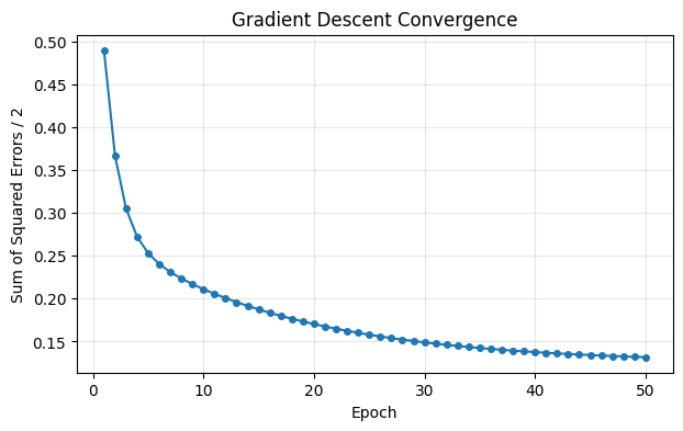
Cost function landscape (3D)
We fix the bias to its final value and plot cost as a function of (w₁, w₂).
This is a simplification — the real landscape lives in 3D (w₁, w₂, b) — but it gives a clear picture of the "valley" that gradient descent navigates.
def cost_for_weights(w1, w2, b, X, y):
    output = X @ np.array([w1, w2]) + b
    return np.log1p(0.5 * ((y - output) ** 2).sum())

b_final = model.b_
w_final = model.w_

w1_range = np.linspace(w_final[0] - 0.5, w_final[0] + 0.5, 60)
w2_range = np.linspace(w_final[1] - 0.5, w_final[1] + 0.5, 60)
W1, W2 = np.meshgrid(w1_range, w2_range)
Cost = np.array([cost_for_weights(w1, w2, b_final, X_and, y_and)
                 for w1, w2 in zip(W1.ravel(), W2.ravel())]).reshape(W1.shape)

fig = plt.figure(figsize=(10, 7))
ax = fig.add_subplot(111, projection="3d")
ax.plot_surface(W1, W2, Cost, cmap="viridis", edgecolor="none", alpha=0.8)

# Overlay gradient descent trajectory
w_hist = np.array(model.w_history_)
cost_hist = np.log1p(np.array(model.losses_))
ax.plot(w_hist[:, 0], w_hist[:, 1], cost_hist,
        color="red", marker=".", linewidth=2, markersize=4, label="GD trajectory")
ax.scatter(*w_hist[0], cost_hist[0], color="orange", marker="X", s=100, label="Start")
ax.scatter(*w_hist[-1], cost_hist[-1], color="red", marker="o", s=100, label="End")

ax.set_xlabel("w₁")
ax.set_ylabel("w₂")
ax.set_zlabel("Cost (log scale)")
ax.set_title("Cost landscape with gradient descent trajectory")
ax.legend()
plt.show()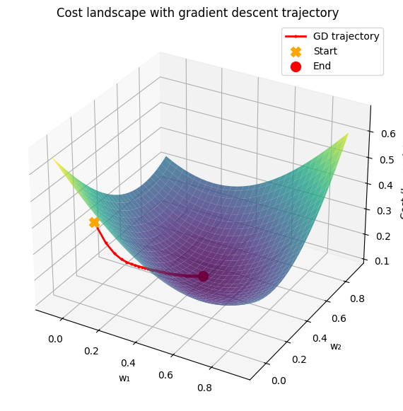
The trajectory shows gradient descent sliding down the cost valley. With a well-chosen learning rate, it converges smoothly to the minimum.
PyTorch comparison
The same ADALINE in PyTorch requires zero manual gradient math — loss.backward() + optimizer.step() handle everything:
import torch
import torch.nn as nn

X_t = torch.FloatTensor(X_and)
y_t = torch.FloatTensor(y_and).unsqueeze(1)

torch_model = nn.Linear(2, 1)
optimizer = torch.optim.SGD(torch_model.parameters(), lr=0.05)
criterion = nn.MSELoss(reduction="sum")

losses_pt = []
for epoch in range(50):
    optimizer.zero_grad()
    loss = 0.5 * criterion(torch_model(X_t), y_t)
    loss.backward()
    optimizer.step()
    losses_pt.append(loss.item())

plt.figure(figsize=(7, 4))
plt.plot(model.losses_, label="NumPy ADALINE", marker="o", markersize=4)
plt.plot(losses_pt, label="PyTorch nn.Linear", marker="s", markersize=4)
plt.xlabel("Epoch")
plt.ylabel("Loss")
plt.title("NumPy vs PyTorch — same algorithm, same result")
plt.legend()
plt.grid(True, alpha=0.3)
plt.show()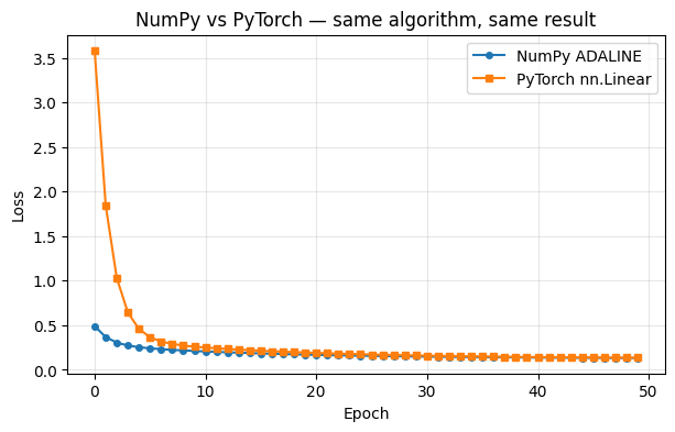
The curves may differ slightly due to different random initialization, but the convergence behavior is identical: both are plain batch gradient descent on MSE loss.
The key takeaway: PyTorch autograd replaces manual gradient derivation. You define the forward pass and the loss, and PyTorch computes all gradients automatically via backpropagation.
What to take away
- Gradient descent updates weights in the direction that reduces the loss: .
- The learning rate () controls step size — too large diverges, too small is slow.
- The cost landscape for a linear model is convex (one minimum) — but for deep networks it has many local minima.
- PyTorch's autograd eliminates the need for manual gradient derivation, making it trivial to train much more complex models.