TensorFlow Playground: Hands-on Guide

Notebook de Jupyter, 4 min de lectura.pytorch/01-deep-learning-fundamentals/complementary/tf_playground_guide.ipynb

En esta página

Playground controls
Experiment 1: linear separation (one neuron)
Experiment 2: non-linear data requires hidden layers
Experiment 3: activation functions
Experiment 4: feature engineering
Experiment 5: learning rate
Experiment 6: overfitting and regularization
Challenge: solve the spiral
Summary

TensorFlow Playground is a web app that lets you configure a small neural network and see it learn in real time on synthetic 2D datasets.

This notebook walks through a series of experiments you can run in the Playground, each illustrating a key concept. For each experiment we also show the equivalent PyTorch code so you can connect the visual intuition with real implementation.

How to use this notebook: open playground.tensorflow.org in a separate tab and follow the experiment instructions. Then run the PyTorch cells to see the same behavior in code.

Playground controls

Control	What it does
Dataset (left panel)	Choose a pattern: two clusters, circle, XOR, spiral
Features	Toggle input transformations: $x_1^2$ , $x_2^2$ , $x_1 \times x_2$ , sin, cos
Hidden layers	Add/remove layers and neurons per layer
Activation	ReLU, Tanh, Sigmoid, or Linear
Learning rate	Step size for the optimizer
Regularization	None, L1, or L2 (with strength slider)
Problem type	Classification or Regression
Play / Pause / Reset	Control training

The colored background shows the decision boundary: blue where the network predicts one class, orange for the other. Line thickness between neurons indicates weight magnitude.

Experiment 1: linear separation (one neuron)

Setup in Playground:

Select the two clusters dataset.
Use only X₁ and X₂ inputs (no extra features).
Remove all hidden layers — just a direct connection to the output.
Press Play.

What you should see: a straight line gradually adjusts to separate the blue and orange points. The loss drops to near zero.

Key insight: a single neuron = a linear classifier. It can only draw one straight boundary.

import torch
import torch.nn as nn
import numpy as np
import matplotlib.pyplot as plt
from sklearn.datasets import make_blobs

# Equivalent: one neuron for linearly separable data
X, y = make_blobs(n_samples=200, centers=2, random_state=42, cluster_std=1.5)
X_t = torch.FloatTensor(X)
y_t = torch.FloatTensor(y).unsqueeze(1)

model = nn.Sequential(nn.Linear(2, 1), nn.Sigmoid())
optimizer = torch.optim.SGD(model.parameters(), lr=0.1)
criterion = nn.BCELoss()

for _ in range(200):
    optimizer.zero_grad()
    criterion(model(X_t), y_t).backward()
    optimizer.step()

# Plot decision boundary
xx, yy = np.meshgrid(np.linspace(X[:, 0].min() - 1, X[:, 0].max() + 1, 200),
                     np.linspace(X[:, 1].min() - 1, X[:, 1].max() + 1, 200))
grid = torch.FloatTensor(np.c_[xx.ravel(), yy.ravel()])
with torch.no_grad():
    Z = model(grid).reshape(xx.shape).numpy()

plt.figure(figsize=(5, 5))
plt.contourf(xx, yy, Z, levels=25, cmap="RdBu", alpha=0.6)
plt.scatter(X[:, 0], X[:, 1], c=y, cmap="RdBu", edgecolors="k", s=30)
plt.title("One neuron → linear boundary")
plt.show()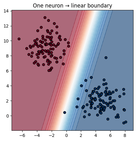

Experiment 2: non-linear data requires hidden layers

Setup in Playground:

Select the circle dataset.
Start with no hidden layers and press Play. Observe that a single neuron fails.
Add a hidden layer with 4 neurons (ReLU or Tanh activation).
Reset and press Play again.

What you should see: with the hidden layer, the boundary curves around the inner circle. Without it, the model is stuck drawing a straight line.

Key insight: hidden layers + activation functions enable non-linear decision boundaries.

from sklearn.datasets import make_circles

X_c, y_c = make_circles(n_samples=300, noise=0.1, factor=0.4, random_state=42)
X_ct = torch.FloatTensor(X_c)
y_ct = torch.FloatTensor(y_c).unsqueeze(1)

# Model with hidden layer
model = nn.Sequential(
    nn.Linear(2, 4), nn.ReLU(),
    nn.Linear(4, 1), nn.Sigmoid(),
)
optimizer = torch.optim.Adam(model.parameters(), lr=0.05)
criterion = nn.BCELoss()

for _ in range(500):
    optimizer.zero_grad()
    criterion(model(X_ct), y_ct).backward()
    optimizer.step()

xx, yy = np.meshgrid(np.linspace(-1.5, 1.5, 200), np.linspace(-1.5, 1.5, 200))
grid = torch.FloatTensor(np.c_[xx.ravel(), yy.ravel()])
with torch.no_grad():
    Z = model(grid).reshape(xx.shape).numpy()

plt.figure(figsize=(5, 5))
plt.contourf(xx, yy, Z, levels=25, cmap="RdBu", alpha=0.6)
plt.scatter(X_c[:, 0], X_c[:, 1], c=y_c, cmap="RdBu", edgecolors="k", s=20)
plt.title("Hidden layer → non-linear boundary")
plt.show()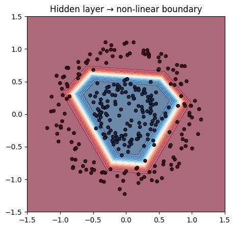

Experiment 3: activation functions

Setup in Playground:

Use the XOR dataset with 1 hidden layer (4 neurons).
Try each activation: ReLU, Tanh, Sigmoid, Linear.
Compare convergence speed and final boundary shape.

Expected results:

ReLU / Tanh: converge relatively fast, good non-linear boundary.
Sigmoid: can be slower due to saturation (gradients shrink for extreme inputs).
Linear: fails — linear(linear) = linear, no non-linearity is introduced.

Key insight: the activation function is what breaks linearity. Without it, adding layers does nothing useful.

# Compare activations on XOR
from sklearn.datasets import make_moons

X_m, y_m = make_moons(n_samples=300, noise=0.15, random_state=42)
X_mt = torch.FloatTensor(X_m)
y_mt = torch.FloatTensor(y_m).unsqueeze(1)

activations = {"ReLU": nn.ReLU(), "Tanh": nn.Tanh(), "Sigmoid": nn.Sigmoid()}
histories = {}

for name, act in activations.items():
    model = nn.Sequential(nn.Linear(2, 8), act, nn.Linear(8, 1))
    opt = torch.optim.Adam(model.parameters(), lr=0.01)
    crit = nn.BCEWithLogitsLoss()
    losses = []
    for _ in range(300):
        opt.zero_grad()
        loss = crit(model(X_mt), y_mt)
        loss.backward()
        opt.step()
        losses.append(loss.item())
    histories[name] = losses

plt.figure(figsize=(8, 4))
for name, losses in histories.items():
    plt.plot(losses, label=name)
plt.xlabel("Epoch")
plt.ylabel("Loss")
plt.title("Activation function comparison")
plt.legend()
plt.show()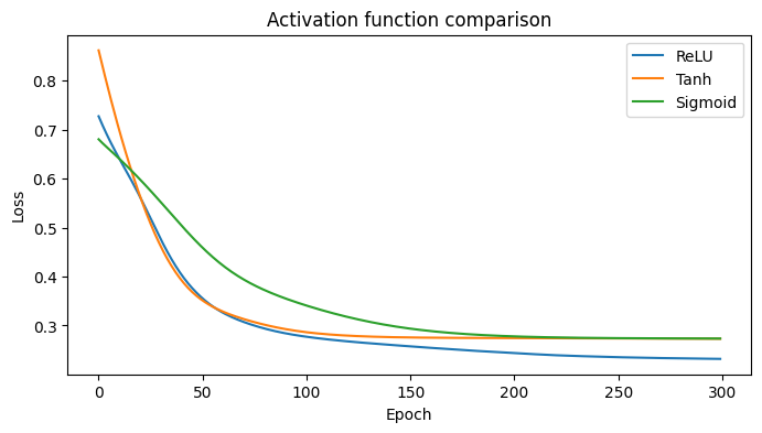

Experiment 4: feature engineering

Setup in Playground:

Select the XOR dataset.
Enable the x₁ × x₂ feature. Remove all hidden layers.
Press Play.

What you should see: XOR is solved with just one neuron! The multiplication feature transforms the problem into something linearly separable.

Key insight: sometimes a well-chosen input feature can replace an entire hidden layer. In deep learning, the network learns these transformations automatically — but sometimes adding domain-specific features helps.

See ➜ complementary/xor_linearity.ipynb for a detailed exploration.

Experiment 5: learning rate

Setup in Playground:

Use the circle dataset with 1 hidden layer (4 neurons, Tanh).
Try learning rates: 0.001, 0.03, 1.0.
Observe training speed and stability.

LR	Effect
0.001	Very slow convergence — loss barely moves
0.03	Stable, steady convergence
1.0	Loss oscillates wildly or diverges

Key insight: the learning rate is the most important hyperparameter to tune. Too high → unstable. Too low → wastes time.

Experiment 6: overfitting and regularization

Setup in Playground:

Select the spiral dataset with high noise.
Use a large network: 2 hidden layers, 8 neurons each, ReLU.
Train without regularization — observe the wiggly boundary.
Now apply L2 regularization (strength ~0.1) — the boundary smooths out.

What's happening: without regularization, the model fits every noisy point. L2 penalizes large weights, forcing simpler (smoother) boundaries.

See ➜ 04_training_dynamics.ipynb for a deeper dive into regularization.

Challenge: solve the spiral

Task: configure a network in TensorFlow Playground that cleanly separates the spiral dataset.

Hints:

You'll likely need 2–3 hidden layers with 6–8 neurons each.
ReLU tends to work well here.
A moderate learning rate (0.01–0.03) is a good starting point.
If the boundary is too wiggly, add some L2 regularization.

Reflect: what was the simplest architecture that worked? How did the learning rate and regularization affect the result?

Summary

Concept	Playground experiment	Takeaway
Linear classifier	One neuron, two clusters	A single neuron draws a straight line
Non-linearity	Circle dataset + hidden layer	Hidden layers enable curved boundaries
Activation functions	XOR + different activations	Non-linear activation is essential
Feature engineering	XOR + x₁×x₂ feature	Good features can replace model complexity
Learning rate	Circle + varying LR	Most important hyperparameter
Regularization	Spiral + L2	Prevents overfitting, smooths boundaries

All of these concepts translate directly to real PyTorch models — the Playground just makes them visible.