PyTorch basics

Notebook de Jupyter, 6 min de lectura.pytorch/01-deep-learning-fundamentals/02_pytorch_basics.ipynb

En esta página

The modern deep learning ecosystem
The two pillars: PyTorch and TensorFlow
Specialized roles
Framework adoption over time
Installation
Tensors
Creating tensors
Operations
Indexing
GPU usage
Building models with nn.Module
Functional style: torch.nn.functional
nn.Sequential
Linear layers in depth
Dataset and DataLoader
Sources

The modern deep learning ecosystem

To understand the current ML landscape, it helps to see the major frameworks as specialized tools for different stages of development.

The two pillars: PyTorch and TensorFlow

	PyTorch (Meta)	TensorFlow (Google)
Strength	Research & Generative AI	Enterprise production
Design	Dynamic graph, Pythonic	Static graph, scalable serving
Key tools	`torch.compile` (2.x), Hugging Face	TF Serving, TF Lite
User base	Academia, LLM/diffusion researchers	Large-scale industry pipelines

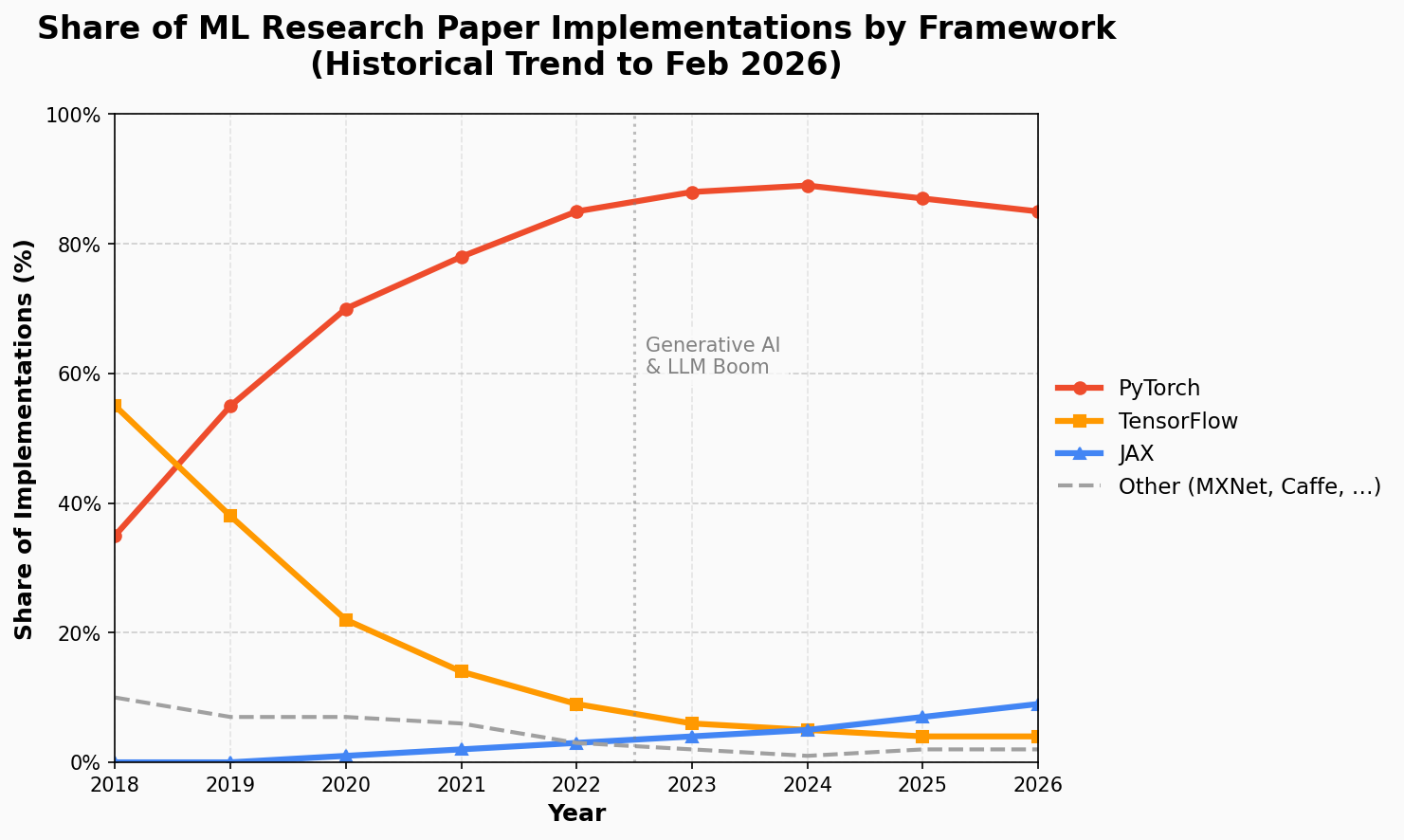
PyTorch is the dominant framework in research and generative AI. Its intuitive, Pythonic design and dynamic computation graph make it the go-to for prototyping new architectures. With PyTorch 2.x and torch.compile, it has also closed the performance gap for production.

TensorFlow remains an enterprise powerhouse — TF Serving and TF Lite keep it entrenched in production pipelines where stability and scalability matter.

Specialized roles

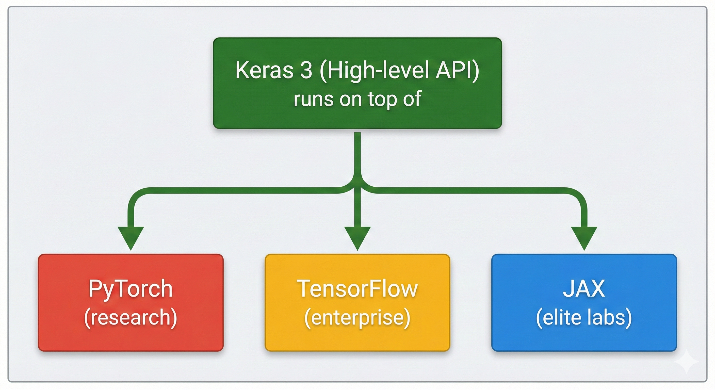
JAX (Google) is a high-performance numerical computing framework used by elite research labs (DeepMind, Anthropic) for training massive models on TPU clusters. Its functional programming style keeps it out of mainstream beginner courses.

Keras 3 is the great unifier: a high-level API that runs on PyTorch, TensorFlow, or JAX. Write once, switch backends.

Framework adoption over time

Installation

Follow the official instructions to install PyTorch for your platform. The installer lets you choose the compute backend:

NVIDIA GPUs: install with CUDA support
AMD GPUs (Linux): use ROCm
Apple Silicon: MPS (Metal Performance Shaders) is built in
CPU only: works everywhere, just slower

With uv: uv add torch torchvision

import torch

print(f"PyTorch version: {torch.__version__}")
print(f"CUDA available: {torch.cuda.is_available()}")

PyTorch version: 2.10.0+cu128
CUDA available: False

Tensors

Tensors are the fundamental data structure in PyTorch — multidimensional arrays, like NumPy arrays, but with two superpowers:

GPU acceleration: tensors can live on CPU or GPU, enabling parallel computation
Automatic differentiation: PyTorch tracks operations on tensors to compute gradients

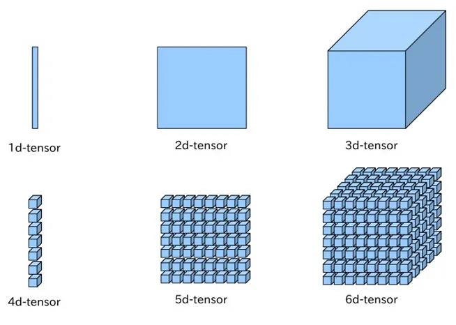
Tensors can represent many types of data:

Scalar (0D): a single number
Vector (1D): a list of features
Matrix (2D): a batch of feature vectors, or a grayscale image
3D tensor: an RGB image (channels × height × width)
4D tensor: a batch of images (batch × channels × height × width)

Creating tensors

import torch
import numpy as np

# From a Python list
t1 = torch.tensor([[1, 2, 3], [4, 5, 6]])
print(f"Tensor:\n{t1}")
print(f"Type: {t1.dtype}")   # int64 (inferred)
print(f"Shape: {t1.shape}")  # torch.Size([2, 3])

Tensor:
tensor([[1, 2, 3],
        [4, 5, 6]])
Type: torch.int64
Shape: torch.Size([2, 3])

# From NumPy (shares memory — changes in one affect the other)
arr = np.array([1.0, 2.0, 3.0])
t_from_np = torch.from_numpy(arr)
print(f"From NumPy: {t_from_np}")

From NumPy: tensor([1., 2., 3.], dtype=torch.float64)

# Common creation functions (same API as NumPy)
print("Zeros:", torch.zeros(2, 3))
print("Ones:", torch.ones(2, 3))
print("Random:", torch.rand(2, 3))
print("Range:", torch.arange(0, 10, 2))

Zeros: tensor([[0., 0., 0.],
        [0., 0., 0.]])
Ones: tensor([[1., 1., 1.],
        [1., 1., 1.]])
Random: tensor([[0.5861, 0.0414, 0.3920],
        [0.1576, 0.1237, 0.4569]])
Range: tensor([0, 2, 4, 6, 8])

# Explicit dtype
t_float = torch.tensor([1, 2, 3], dtype=torch.float32)
print(f"float32 tensor: {t_float}")

float32 tensor: tensor([1., 2., 3.])

Operations

a = torch.tensor([[1, 2], [3, 4]], dtype=torch.float32)
b = torch.tensor([[5, 6], [7, 8]], dtype=torch.float32)

# Element-wise operations
print("a + b =", a + b)
print("a * b =", a * b)

# Matrix multiplication (two equivalent ways)
print("a @ b =", a @ b)
print("matmul:", torch.matmul(a, b))

# Transpose
print("a.T =", a.T)

a + b = tensor([[ 6.,  8.],
        [10., 12.]])
a * b = tensor([[ 5., 12.],
        [21., 32.]])
a @ b = tensor([[19., 22.],
        [43., 50.]])
matmul: tensor([[19., 22.],
        [43., 50.]])
a.T = tensor([[1., 3.],
        [2., 4.]])

Indexing

t = torch.tensor([[10, 20, 30], [40, 50, 60], [70, 80, 90]])

print("First row:", t[0])
print("Element [1,2]:", t[1, 2])
print("Second column:", t[:, 1])
print("Submatrix:", t[1:, 1:])

First row: tensor([10, 20, 30])
Element [1,2]: tensor(60)
Second column: tensor([20, 50, 80])
Submatrix: tensor([[50, 60],
        [80, 90]])

GPU usage

GPUs dramatically accelerate neural network training through massive parallelism (GPGPU — General-Purpose computing on Graphics Processing Units).

PyTorch natively supports:

NVIDIA GPUs via CUDA
Apple Silicon via Metal (MPS)
AMD GPUs via ROCm

Tensors must be on the same device before you can combine them:

device = (
    "cuda" if torch.cuda.is_available()
    else "mps" if torch.backends.mps.is_available()
    else "cpu"
)
print(f"Using device: {device}")

if device == "cuda":
    print(f"GPU: {torch.cuda.get_device_name(0)}")

Using device: cpu

# Moving tensors between devices
t_cpu = torch.rand(3, 3)
print(f"Device: {t_cpu.device}")

t_device = t_cpu.to(device)
print(f"After .to('{device}'): {t_device.device}")

# Operations require same device — this would fail:
# torch.matmul(t_cpu, t_device)  # RuntimeError!

# Move both to the same device first
result = torch.matmul(t_cpu.to(device), t_device)
print(f"Result on {result.device}: {result}")

Device: cpu
After .to('cpu'): cpu
Result on cpu: tensor([[0.3309, 0.4180, 0.3443],
        [0.7214, 0.6000, 0.7555],
        [0.9673, 0.5034, 0.7142]])

Building models with `nn.Module`

torch.nn.Module is the base class for every neural network in PyTorch. To create a model, you:

Subclass nn.Module
Define layers in __init__
Define how data flows through in forward

PyTorch automatically tracks all nn.Parameter objects (weights, biases) registered in __init__, so you can iterate over them with .parameters():

import torch.nn as nn

class TinyModel(nn.Module):
    def __init__(self):
        super().__init__()
        self.linear1 = nn.Linear(100, 200)
        self.activation = nn.ReLU()
        self.linear2 = nn.Linear(200, 10)

    def forward(self, x: torch.Tensor) -> torch.Tensor:
        x = self.linear1(x)
        x = self.activation(x)
        x = self.linear2(x)
        return x

model = TinyModel()
print(model)
print(f"\nTotal parameters: {sum(p.numel() for p in model.parameters()):,}")

TinyModel(
  (linear1): Linear(in_features=100, out_features=200, bias=True)
  (activation): ReLU()
  (linear2): Linear(in_features=200, out_features=10, bias=True)
)

Total parameters: 22,210

# You can inspect individual layers and their parameters
print("Just the second layer:")
print(model.linear2)
print(f"  Weight shape: {model.linear2.weight.shape}")
print(f"  Bias shape:   {model.linear2.bias.shape}")

Just the second layer:
Linear(in_features=200, out_features=10, bias=True)
  Weight shape: torch.Size([10, 200])
  Bias shape:   torch.Size([10])

Functional style: `torch.nn.functional`

The torch.nn.functional module provides the same operations as module-based layers, but as stateless functions. This is useful for operations without learnable parameters (like activations):

import torch.nn.functional as F

class TinyModelFunctional(nn.Module):
    def __init__(self):
        super().__init__()
        self.linear1 = nn.Linear(100, 200)
        self.linear2 = nn.Linear(200, 10)

    def forward(self, x: torch.Tensor) -> torch.Tensor:
        x = F.relu(self.linear1(x))  # Functional activation
        x = self.linear2(x)
        return x

# Both styles produce the same result — it's a matter of preference

In this case, the nn.functional library is used to call activation functions directly. It's another programming style. In both cases they are called from forward, but the difference is that in this case there's no need to create a class attribute nn.ReLU() in the constructor.

`nn.Sequential`

For simple models where layers are applied one after another, nn.Sequential saves boilerplate. You don't even need a forward method:

# These three definitions are equivalent:

# 1. Sequential (simplest)
model_seq = nn.Sequential(
    nn.Linear(100, 200),
    nn.ReLU(),
    nn.Linear(200, 10),
)

# 2. Sequential with named layers (useful for debugging)
from collections import OrderedDict

model_named = nn.Sequential(OrderedDict([
    ("fc1", nn.Linear(100, 200)),
    ("relu", nn.ReLU()),
    ("fc2", nn.Linear(200, 10)),
]))

# Both work the same way:
x = torch.rand(1, 100)
print(f"Sequential output shape: {model_seq(x).shape}")
print(f"Named output shape:      {model_named(x).shape}")

Sequential output shape: torch.Size([1, 10])
Named output shape:      torch.Size([1, 10])

Linear layers in depth

A linear (fully connected) layer computes:

$y = xW^T + b$

where $W$ is the weight matrix and $b$ is the bias vector. If the layer has $m$ inputs and $n$ outputs, then $W$ has shape $(n, m)$ and $b$ has shape $(n,)$ .

For example, with 3 inputs and 2 outputs:

$\begin{bmatrix} y_1 \\ y_2 \end{bmatrix} = \begin{bmatrix} w_{11} & w_{12} & w_{13} \\ w_{21} & w_{22} & w_{23} \end{bmatrix} \begin{bmatrix} x_1 \\ x_2 \\ x_3 \end{bmatrix} + \begin{bmatrix} b_1 \\ b_2 \end{bmatrix}$

# Verify the math manually
lin = nn.Linear(3, 2)

x = torch.tensor([[1.0, 2.0, 3.0]])
y = lin(x)

# Manual computation: y = x @ W^T + b
y_manual = x @ lin.weight.T + lin.bias
print(f"Layer output:  {y.detach()}")
print(f"Manual output: {y_manual.detach()}")
print(f"Match: {torch.allclose(y, y_manual)}")

Layer output:  tensor([[-0.0194,  0.9717]])
Manual output: tensor([[-0.0194,  0.9717]])
Match: True

Dataset and DataLoader

PyTorch provides two key abstractions for data handling:

torch.utils.data.Dataset: represents a collection of samples. Must implement __len__ and __getitem__.
torch.utils.data.DataLoader: wraps a Dataset and provides batching, shuffling, and parallel loading.

This is how you feed data to your training loop:

from torch.utils.data import Dataset, DataLoader

# A minimal custom dataset
class SyntheticDataset(Dataset):
    def __init__(self, n_samples: int = 1000, n_features: int = 10):
        self.X = torch.randn(n_samples, n_features)
        self.y = (self.X.sum(dim=1) > 0).long()  # Binary label

    def __len__(self) -> int:
        return len(self.X)

    def __getitem__(self, idx: int) -> tuple[torch.Tensor, torch.Tensor]:
        return self.X[idx], self.y[idx]

dataset = SyntheticDataset(n_samples=200)
print(f"Dataset size: {len(dataset)}")
print(f"One sample: X shape={dataset[0][0].shape}, y={dataset[0][1]}")

Dataset size: 200
One sample: X shape=torch.Size([10]), y=1

# DataLoader: handles batching and shuffling
loader = DataLoader(dataset, batch_size=32, shuffle=True)

# Iterate over one batch
batch_X, batch_y = next(iter(loader))
print(f"Batch X shape: {batch_X.shape}")  # (32, 10)
print(f"Batch y shape: {batch_y.shape}")  # (32,)
print(f"Labels in batch: {batch_y}")

Batch X shape: torch.Size([32, 10])
Batch y shape: torch.Size([32])
Labels in batch: tensor([0, 0, 0, 1, 0, 0, 0, 1, 1, 1, 1, 1, 0, 0, 1, 0, 0, 1, 0, 1, 1, 1, 0, 1,
        1, 1, 0, 1, 0, 0, 1, 1])

Key parameters:

batch_size: how many samples per batch (32-256 is typical)
shuffle=True: randomize order each epoch (important for training, not for evaluation)
num_workers: parallel data loading processes (set to 0 on Windows/macOS, 2-4 on Linux)

PyTorch also provides ready-made datasets (MNIST, FashionMNIST, CIFAR-10, …) via torchvision.datasets. We'll use one in the next notebook.