Training Dynamics: Loss Functions, Optimizers, and Regularization
En esta página
The training landscape
Training a neural network means navigating a high-dimensional loss surface to find parameters that generalize well.
Three knobs control this process:
- Loss function — what we minimize (defines the objective)
- Optimizer — how we update weights (the step strategy)
- Regularization — constraints that prevent memorizing noise
We will explore each one with runnable experiments on a small 2D dataset.
Toy dataset: make_moons
We use make_moons from scikit-learn — a 2-class dataset that is not linearly separable but simple enough to visualize.
import torch
import torch.nn as nn
import torch.optim as optim
import matplotlib.pyplot as plt
import numpy as np
from sklearn.datasets import make_moons
from sklearn.model_selection import train_test_split

X, y = make_moons(n_samples=300, noise=0.2, random_state=42)
X_train, X_val, y_train, y_val = train_test_split(X, y, test_size=0.3, random_state=42)

X_train_t = torch.FloatTensor(X_train)
y_train_t = torch.FloatTensor(y_train).unsqueeze(1)
X_val_t = torch.FloatTensor(X_val)
y_val_t = torch.FloatTensor(y_val).unsqueeze(1)

fig, axes = plt.subplots(1, 2, figsize=(10, 4))
for ax, (Xp, title) in zip(axes, [(X_train, "Training set"), (X_val, "Validation set")]):
    ax.scatter(Xp[y_train == 0 if "Train" in title else y_val == 0, 0],
               Xp[y_train == 0 if "Train" in title else y_val == 0, 1],
               s=15, alpha=0.7, label="class 0")
    ax.scatter(Xp[y_train == 1 if "Train" in title else y_val == 1, 0],
               Xp[y_train == 1 if "Train" in title else y_val == 1, 1],
               s=15, alpha=0.7, label="class 1")
    ax.set_title(title)
    ax.legend()
plt.tight_layout()
plt.show()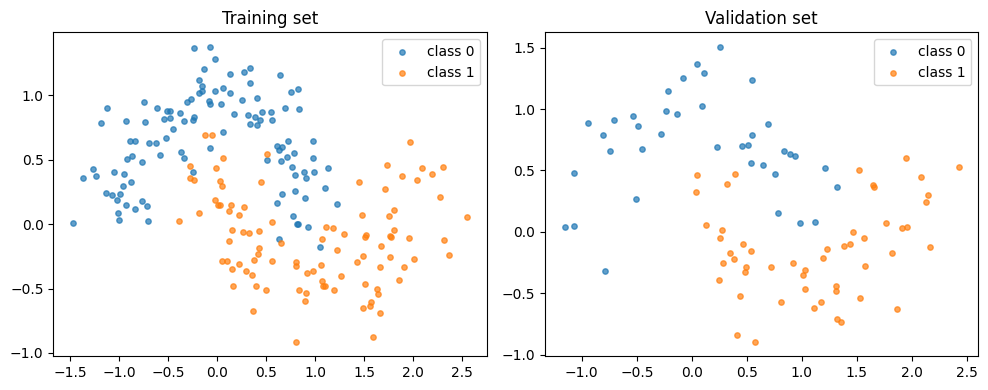
Loss functions
The loss function quantifies how wrong the model's predictions are.
| Task | Loss | PyTorch | Notes |
|---|---|---|---|
| Regression | Mean Squared Error | nn.MSELoss() | Penalizes large errors quadratically |
| Binary classification | Binary Cross-Entropy | nn.BCEWithLogitsLoss() | Expects raw logits (more numerically stable than nn.BCELoss + sigmoid) |
| Multi-class classification | Cross-Entropy | nn.CrossEntropyLoss() | Expects raw logits, applies softmax internally |
Rule of thumb: for classification, always use the WithLogits / CrossEntropy variants and let PyTorch apply sigmoid/softmax internally — this avoids numerical issues with log(0).
Quick demo: BCE loss on make_moons
We train the same small model with BCEWithLogitsLoss — the standard choice for binary problems.
model = nn.Sequential(nn.Linear(2, 16), nn.ReLU(), nn.Linear(16, 1))
criterion = nn.BCEWithLogitsLoss()
optimizer = optim.Adam(model.parameters(), lr=0.01)

losses = []
for epoch in range(300):
    optimizer.zero_grad()
    loss = criterion(model(X_train_t), y_train_t)
    loss.backward()
    optimizer.step()
    losses.append(loss.item())

plt.figure(figsize=(6, 3))
plt.plot(losses)
plt.xlabel("Epoch")
plt.ylabel("BCE Loss")
plt.title("Training loss curve")
plt.show()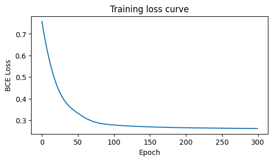
Optimizers
All optimizers follow the same idea: update weights in the direction that reduces the loss. They differ in how they calculate the step.
| Optimizer | Intuition | When to use |
|---|---|---|
SGD | "Walk downhill" — follows the raw gradient | Baseline, good for convex problems |
SGD + momentum | "Ball rolling downhill" — accumulates velocity | Faster convergence, escapes shallow local minima |
RMSprop | "Adaptive step size" — scales LR per parameter | Good for non-stationary objectives (e.g. RNNs) |
Adam | Combines momentum + adaptive LR | Default choice for most deep learning problems |
Practical recommendation: start with Adam(lr=1e-3). If you need to squeeze the last %, switch to SGD + momentum with a learning rate schedule.
Want to see optimizers in action? Open ➜ complementary/tf_playground_guide.ipynb and experiment with different learning rates interactively.
Comparison experiment
def train_with_optimizer(opt_fn, lr, epochs=500):
    model = nn.Sequential(nn.Linear(2, 64), nn.ReLU(), nn.Linear(64, 64), nn.ReLU(), nn.Linear(64, 1))
    optimizer = opt_fn(model.parameters(), lr=lr)
    criterion = nn.BCEWithLogitsLoss()
    losses = []
    for _ in range(epochs):
        optimizer.zero_grad()
        loss = criterion(model(X_train_t), y_train_t)
        loss.backward()
        optimizer.step()
        losses.append(loss.item())
    return losses

configs = [
    (lambda p, lr: optim.SGD(p, lr=lr), 0.1, "SGD"),
    (lambda p, lr: optim.SGD(p, lr=lr, momentum=0.9), 0.01, "SGD + Momentum"),
    (lambda p, lr: optim.Adam(p, lr=lr), 0.01, "Adam"),
]

plt.figure(figsize=(10, 5))
for opt_fn, lr, name in configs:
    losses = train_with_optimizer(opt_fn, lr)
    plt.plot(losses, label=name)
plt.xlabel("Epoch")
plt.ylabel("Loss (BCE)")
plt.yscale("log")
plt.title("Optimizer comparison on make_moons")
plt.legend()
plt.show()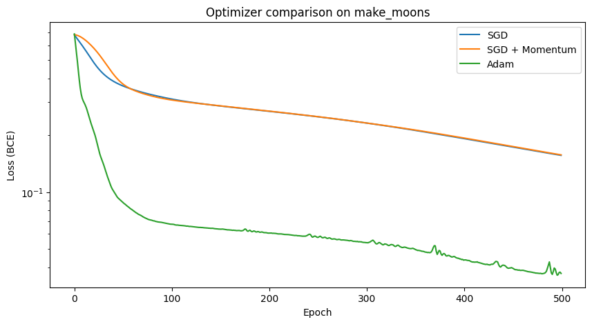
What to observe:
- SGD converges slowly and may plateau early.
- SGD + Momentum accelerates past flat regions.
- Adam typically reaches a low loss fastest thanks to adaptive learning rates.
Overfitting and regularization
Overfitting happens when the model memorizes the training data (including noise) instead of learning the underlying pattern.
Tell-tale sign: training loss keeps decreasing while validation loss starts increasing.
Three common defenses:
| Technique | How it works | PyTorch |
|---|---|---|
| Weight decay (L2) | Penalizes large weights — shrinks them towards zero | Adam(..., weight_decay=1e-4) |
| Dropout | Randomly zeros neurons during training — forces redundancy | nn.Dropout(p=0.5) |
| Early stopping | Stop training when validation loss stops improving | Manual check in training loop |
Experiment: baseline vs. regularized
class FlexibleModel(nn.Module):
    def __init__(self, dropout: float = 0.0):
        super().__init__()
        self.net = nn.Sequential(
            nn.Linear(2, 128), nn.ReLU(), nn.Dropout(dropout),
            nn.Linear(128, 128), nn.ReLU(), nn.Dropout(dropout),
            nn.Linear(128, 1),
        )

    def forward(self, x):
        return self.net(x)

def train_and_record(model, weight_decay: float = 0.0, epochs: int = 1000):
    optimizer = optim.Adam(model.parameters(), lr=0.01, weight_decay=weight_decay)
    criterion = nn.BCEWithLogitsLoss()
    train_losses, val_losses = [], []

    for _ in range(epochs):
        model.train()
        optimizer.zero_grad()
        loss = criterion(model(X_train_t), y_train_t)
        loss.backward()
        optimizer.step()
        train_losses.append(loss.item())

        model.eval()
        with torch.no_grad():
            val_loss = criterion(model(X_val_t), y_val_t)
            val_losses.append(val_loss.item())
    return train_losses, val_losses

# Baseline (overparameterized, no regularization)
baseline = FlexibleModel(dropout=0.0)
bl_train, bl_val = train_and_record(baseline, weight_decay=0.0)

# Regularized (dropout + weight decay)
regularized = FlexibleModel(dropout=0.5)
reg_train, reg_val = train_and_record(regularized, weight_decay=1e-3)

fig, axes = plt.subplots(1, 2, figsize=(14, 5))
for ax, (tr, vl, title) in zip(axes, [
    (bl_train, bl_val, "Baseline (no regularization)"),
    (reg_train, reg_val, "Regularized (Dropout + weight decay)"),
]):
    ax.plot(tr, label="Train", linestyle="--")
    ax.plot(vl, label="Validation")
    ax.set_xlabel("Epoch")
    ax.set_ylabel("Loss")
    ax.set_title(title)
    ax.set_ylim(0, 1.0)
    ax.legend()
plt.tight_layout()
plt.show()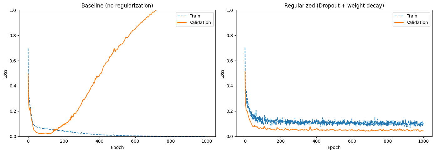
What to observe:
- Baseline: validation loss eventually rises even as training loss drops — classic overfitting.
- Regularized: the gap between train and validation is smaller, showing better generalization.
Learning rate scheduling
The learning rate (LR) is the single most impactful hyperparameter:
- Too high → the loss oscillates or diverges.
- Too low → training is painfully slow.
Schedulers adjust the LR during training, typically starting high and decaying over time.
| Scheduler | Behavior | Use case |
|---|---|---|
StepLR | Multiply LR by γ every N epochs | Simple, reliable |
CosineAnnealingLR | Follows a cosine curve to near-zero | Smooth decay, popular in vision |
ReduceLROnPlateau | Cuts LR when a metric stalls | Doesn't need predefined schedule |
model = nn.Linear(10, 1)
optimizer = optim.SGD(model.parameters(), lr=0.1)

# Three schedulers for comparison
schedulers = {
    "StepLR (step=30, γ=0.1)": optim.lr_scheduler.StepLR(optimizer, step_size=30, gamma=0.1),
}

# Reset and collect LR for StepLR
lrs_step = []
for epoch in range(100):
    optimizer.step()
    lrs_step.append(optimizer.param_groups[0]["lr"])
    schedulers["StepLR (step=30, γ=0.1)"].step()

# CosineAnnealing
optimizer2 = optim.SGD(model.parameters(), lr=0.1)
sched_cos = optim.lr_scheduler.CosineAnnealingLR(optimizer2, T_max=100)
lrs_cos = []
for epoch in range(100):
    optimizer2.step()
    lrs_cos.append(optimizer2.param_groups[0]["lr"])
    sched_cos.step()

plt.figure(figsize=(8, 4))
plt.plot(lrs_step, label="StepLR")
plt.plot(lrs_cos, label="CosineAnnealingLR")
plt.xlabel("Epoch")
plt.ylabel("Learning Rate")
plt.title("Learning rate schedules")
plt.legend()
plt.show()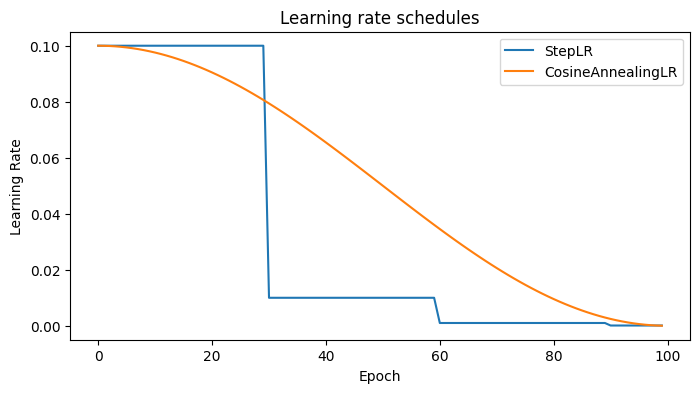
Summary
| Component | Practical default |
|---|---|
| Loss | CrossEntropyLoss (multi-class) or BCEWithLogitsLoss (binary) |
| Optimizer | Adam(lr=1e-3) — switch to SGD + momentum for fine-tuning |
| Regularization | Dropout (0.2–0.5) in hidden layers + small weight_decay |
| LR schedule | ReduceLROnPlateau for robustness, CosineAnnealing for vision |
| Monitoring | Always compare train vs. validation loss to detect overfitting |