NumPy
En esta página
- Introduction
- Sources:
- Installation and importing NumPy
- Installation
- Importing
- Creating arrays from lists
- Data types for array elements
- NaN
- Accessing elements
- Basic functions to create arrays
- Random number generation
- Functions to create vectors following sequences
- Reshape
- Slicing
- Filtering
- Mathematical operations
- Operations on matrices
- Sorting
- Unique
- Flip
- Additional resources
Introduction
NumPy is a Python library that provides functions for working with arrays of 1 (vectors), 2 (matrices), and n dimensions.
NumPy works similarly to Python lists, but with the difference that its arrays are homogeneous (all elements are of the same type) and have a fixed size (cannot be modified once created).
NumPy arrays are more efficient than Python lists, as they are implemented in C++ and execute faster. They use much less memory and allow specifying the data type contained in the array.
It is one of the most widely used libraries in the field of data science and machine learning. Many other libraries use it as a foundation (it is therefore a dependency for them): pandas, Matplotlib, Seaborn, scikit-learn, TensorFlow, PyTorch, Keras...
Sources:
- Official NumPy documentation
- Tutorial for learning NumPy from scratch (most images reference this guide)
Installation and importing NumPy
Installation
To be able to import the NumPy module, it is first necessary to have it installed in our environment.
Depending on which package manager we are using, it can be installed with pip:
pip install numpywith Conda (Anaconda or Miniconda):
conda install numpyor with uv:
uv add numpyImporting
The alias "np" is practically a de facto standard. It is not necessary but we will find it in most examples and documentation.
import numpy as npCreating arrays from lists
# Creating a Python list
python_list_1D=[1, 2, 3, 4, 5, 6]
print(python_list_1D)
print(type(python_list_1D))

# Creating a vector (1D ndarray) from the list
numpy_darray_1D = np.array(python_list_1D)
print(numpy_darray_1D)
print(type(numpy_darray_1D)) # The type of NumPy variables is numpy.ndarray

numpy_darray_1D # Notebooks allow displaying variable content without using print
[1, 2, 3, 4, 5, 6] <class 'list'> [1 2 3 4 5 6] <class 'numpy.ndarray'>
array([1, 2, 3, 4, 5, 6])

python_list_2D=[[1, 2, 3], [4, 5, 6]] # List of lists (2D) in Python
print(python_list_2D)
print(type(python_list_2D))

numpy_darray_2D = np.array(python_list_2D) # Creating a 2D ndarray
print(numpy_darray_2D)
print(type(numpy_darray_2D))
numpy_darray_2D
[[1, 2, 3], [4, 5, 6]] <class 'list'> [[1 2 3] [4 5 6]] <class 'numpy.ndarray'>
array([[1, 2, 3],
       [4, 5, 6]])
numpy_darray_2D = np.array([[1, 2, 3], [4, 5, 6]])
print(numpy_darray_2D)
### Properties of NumPy variables:
print(numpy_darray_2D.ndim) # dimensions of the matrix
print(numpy_darray_2D.shape) # shape of the matrix (number of elements per dimension or axis)
print(numpy_darray_2D.size) # total number of elements
print(numpy_darray_2D.dtype) # type of the matrix elements[[1 2 3] [4 5 6]] 2 (2, 3) 6 int64
Data types for array elements
NumPy array objects are always of type ndarray (N-dimensional array). The type of its elements is specified by its dtype (data type). ndarrays are always homogeneous, meaning all their elements are of the same type.
# If we don't specify the element type, NumPy infers it from the argument
lista = [[1, 2, 3], [4, 5, 6]]
a = np.array(lista)
print(a)
print(a.dtype)

# We can create a NumPy ndarray with elements of a specific type
b = np.array(lista, dtype=np.float64) # 64-bit float
# Although we pass a list with ints, with the dtype parameter we can indicate that we want the elements to be floats, so it converts them. We can see this when displaying it with print by the decimal point.
print(b)
print(b.dtype)
[[1 2 3] [4 5 6]] int64 [[1. 2. 3.] [4. 5. 6.]] float64
# Suppose we use an array like the following to store grades from 2 exams of a class list:
students_and_grades = np.array([['Antonio','Bea','Carlos','Diana'],
                            [65,78,90,81],
                            [71,82,79,92]]) # Do you see anything that could be improved in this data structure?

# Elements within a NumPy array must be of the same type. If we pass a list with elements of different types, NumPy converts them all to the same type. In this case, being strings, it converts them all to strings.
print(students_and_grades)
print(students_and_grades.dtype) # dtype='<U11' means they are Unicode strings of up to 11 characters
[['Antonio' 'Bea' 'Carlos' 'Diana'] ['65' '78' '90' '81'] ['71' '82' '79' '92']] <U21
Apart from the previous example serving to exemplify typing in NumPy, that structure could be improved. Not only does it not fit into NumPy's philosophy (efficient execution of mathematical operations); it wouldn't change much from leaving it as a list of lists:
students_and_grades = [['Antonio', 'Bea', 'Carlos', 'Diana'],
                     [65, 78, 90, 81],
                     [71, 82, 79, 92]]
but rather than linking several lists by their index (which can be a source of errors when deleting or sorting elements synchronously across all of them), it would be recommended to first encapsulate each student with their grades (in a tuple or an object) and maintain a list of them:
students_and_grades = [('Antonio', [65, 71]), ('Bea', [78, 82]), ('Carlos', [90, 79]), ('Diana', [81, 92])]This would be questionable if we need to do costly processing of a large number of student grades, but in that case, it would be recommended to use a more complex data structure, such as a Pandas DataFrame, which would allow us to perform operations efficiently.
NaN
The float data type in NumPy allows the special value NaN (Not a Number), which is used to represent numeric values that are not real numbers while maintaining the float data type to be able to perform operations with them. For example, the result of dividing 0 by 0 is NaN.
If we used the None type to represent numeric values that are not real numbers, the resulting data type would be object, and we couldn't perform mathematical operations with it.
print(type(np.nan))
print(type(None))
<class 'float'> <class 'NoneType'>
np.array([[1, 2, 3], [4, np.nan, 6]])array([[ 1., 2., 3.],
[ 4., nan, 6.]])Accessing elements
numpy_darray_2D[1,1] # Access to an element of the ndarray (row 1, column 1)np.int64(5)
A = np.array([[11, 12, 13, 14], [21, 22, 23, 24], [31, 32, 33, 34]])
A
array([[11, 12, 13, 14],
[21, 22, 23, 24],
[31, 32, 33, 34]])The previous cell defines with NumPy a 3x4 matrix (3 rows and 4 columns) like the following:
To access its values in Python, the syntax A[row, column] is used, remembering that indices start at 0, so the first element of the matrix is accessed with A[0,0] and the last with A[2,3].
print(A[0,0]) # Element of the first row (row 0) and first column (column 0)
print(A[1,2]) # Element of the second row (row 1) and third column (column 2)
print(A[1]) # Second row of A (index 1)
11 23 [21 22 23 24]
Basic functions to create arrays
print(np.zeros(4)) # Creates a NumPy vector with four elements set to 0
print(np.ones(2)) # Creates a NumPy ndarray with two elements set to 1
[0. 0. 0. 0.] [1. 1.]
# The shape parameter allows us to specify the shape of the matrix, receives a tuple with its dimensions
np.zeros(shape=(2,3)) # Creates a 2x3 matrix of zeros. Dimensions (tuple 2,3) with zeros
array([[0., 0., 0.],
[0., 0., 0.]])np.ones((2,2,2), dtype=int) # Creates a 2x2x2 three-dimensional array with ones of type intarray([[[1, 1],
[1, 1]],
[[1, 1],
[1, 1]]])# np.zeros, np.ones default to float64 type, but we can specify the type with the dtype parameter
print(np.zeros(4))
print(np.zeros(4, dtype=np.int64))
print(np.arange(254, 259, dtype=np.uint8)) # In this case, the type is uint8 (unsigned 8-bit int), so the maximum value it can take is 255 and it overflows[0. 0. 0. 0.] [0 0 0 0] [254 255 0 1 2]
# np.empty does not initialize its elements, so they take the value that was in the memory position
np.empty(2)
array([1., 1.])
print(np.full((3,3), True)) # Creates a 3x3 matrix with all elements set to True
print(np.full(shape=(3,2), fill_value=5)) # Creates a 3x2 matrix with all elements set to 5 (int)

# np.full will take the type of the argument we pass to it (like np.array with the elements contained in the sequence passed to it), so if we pass a float, the elements will be floats

print(np.full((3,2), 5.0)) # Creates a 3x2 matrix with all elements set to 5.0
print(np.full((3,2), 5, dtype=np.float64)) # Creates a 3x2 matrix with all elements set to 5.0
[[ True True True] [ True True True] [ True True True]] [[5 5] [5 5] [5 5]] [[5. 5.] [5. 5.] [5. 5.]] [[5. 5.] [5. 5.] [5. 5.]]
Random number generation
rng = np.random.default_rng() # Create a NumPy random number generator
print(rng.random((3, 4))) # Creates a 3x4 matrix with random numbers between 0 and 1
print(rng.integers(5, size=(2, 4))) # Creates a 2x4 matrix with random integers between 0 and 4
[[0.87298025 0.75971036 0.9505646 0.25030904] [0.83941352 0.81611634 0.25656097 0.47025815] [0.37161966 0.82545842 0.19139435 0.25963486]] [[2 1 4 3] [4 1 0 1]]
Functions to create vectors following sequences
print(np.arange(2, 10, 2)) # Same as Python's range function, but returns a NumPy ndarray
print(np.arange(10))
print(np.linspace(0, 10, num=5)) # Returns a NumPy ndarray with 5 evenly spaced elements between 0 and 10
[2 4 6 8] [0 1 2 3 4 5 6 7 8 9] [ 0. 2.5 5. 7.5 10. ]
Reshape
# A vector can be converted into a matrix with the reshape function
base_vector=np.arange(12)
print(base_vector.reshape(3, 4)) # Creates a 12-element vector and converts it into a 3x4 matrix
# In a matrix shape, the first element is the number of rows (axis 0) and the second is the number of columns (axis 1)
[[ 0 1 2 3] [ 4 5 6 7] [ 8 9 10 11]]
# The special value -1 in the shape parameter indicates that NumPy should infer the value of that dimension
print(base_vector.reshape(3, -1)) # Creates a 12-element vector and converts it into a 3x4 matrix
[[ 0 1 2 3] [ 4 5 6 7] [ 8 9 10 11]]
np.array([1, 2, 3]).reshape(-1,1) # Converts a vector into a single-column matrixarray([[1],
[2],
[3]])Slicing
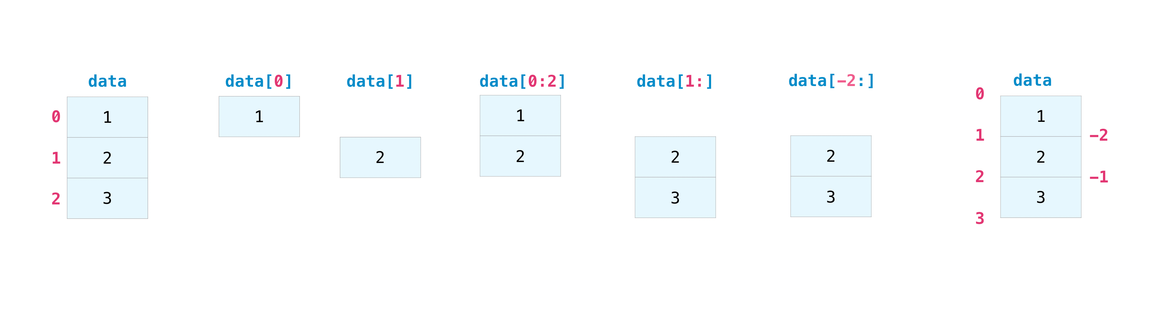
Slicing is a way to retrieve a part of the matrix. It works analogously to Python lists.
a[start:stop]  # elements from start to stop-1 (stop is the first element not included)
a[start:]      # elements from start to the end of the array
a[:stop]       # elements from the beginning of the array to stop-1
a[:]           # a copy of the complete array
There is also a third value, the "step" increment:
a[start:stop:step] # from start to a value less than stop, with increment "step"Start and stop can be negative numbers. That means counting from the end of the array:
a[-1]    # Last element of the array
a[-2:]   # Last two elements of the array
a[:-2]   # All elements of the array except the last two
Step can also be negative:
a[::-1]    # all elements of the array but reversed, starting with the last (equivalent to np.flip(a))
a[1::-1]   # the two elements, reversed
a[:-3:-1]  # the last two elements, reversed
a[-3::-1]  # everything except the last two elements, reversed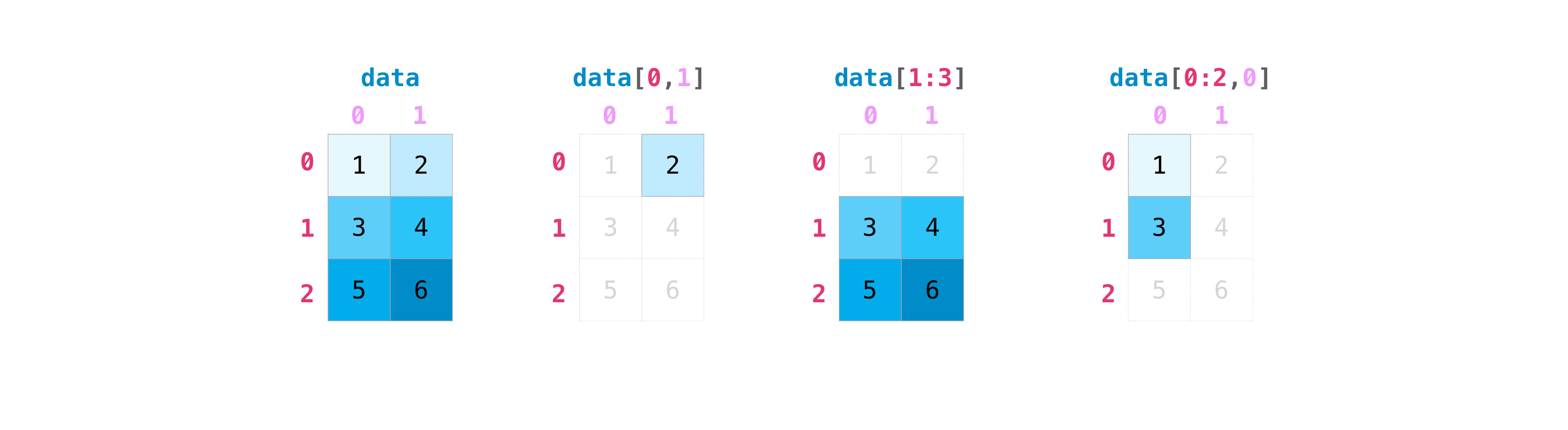
print(f"{A}\n---")

print(f"Row 1: {A[1,:]}") # The row with index 1 and all columns. That is: the 2nd row
print(f"Row 1: {A[1]}") # same as the previous one, simplified
[[11 12 13 14] [21 22 23 24] [31 32 33 34]] --- Row 1: [21 22 23 24] Row 1: [21 22 23 24]
A[:,1] # The elements of all rows (:) and column 1. That is: those of the 2nd column
# A vector with those values is returned (not a matrix with a single column)
array([12, 22, 32])
# Same as the previous one, but returns a single-column matrix
A[:,1:2]
# print(f"Column 1: {A[:,1].reshape(-1,1)}") # Equivalent
array([[12],
[22],
[32]])print(f"{A}\n---")
print(f"Row 1, columns 0 and 1: {A[1,:2]}") # Row 1 and columns 0 and 1 (all up to 2)[[11 12 13 14] [21 22 23 24] [31 32 33 34]] --- Row 1, columns 0 and 1: [21 22]
print(f"{A}\n---")

print(A[1:3,1:3])  # Submatrix of A with rows 1 and 2 and columns 1 and 2
print(A[1:,1:])  # Submatrix of A with rows 1 and 2 and columns 1, 2 and 3
[[11 12 13 14] [21 22 23 24] [31 32 33 34]] --- [[22 23] [32 33]] [[22 23 24] [32 33 34]]
Filtering
arr = np.array([1, 2, 3, 4])
print(arr)
x = [True, False, True, False]
filtered_array = arr[x] # Filter the elements of arr that are in the True positions of x
print(filtered_array)
[1 2 3 4] [1 3]
a = np.arange(11)**2
print(a)
print(a[a<10]) # Keep values less than 10
print(a[a==16]) # Keep values equal to 16
print(a[a!=16]) # Keep values different from 16
print(a[(a>20) | (a<50)]) # Keep values greater than 20 or less than 50
print(a[(a>20) & (a<50)]) # Keep values greater than 20 and less than 50
[ 0 1 4 9 16 25 36 49 64 81 100] [0 1 4 9] [16] [ 0 1 4 9 25 36 49 64 81 100] [ 0 1 4 9 16 25 36 49 64 81 100] [25 36 49]
# Starting from filters we can make modifications on certain elements of an ndarray
a[a<10] = 0 # Set values less than 10 to 0
print(a)

b = np.arange(12).reshape(3,4)
print(b)
# Set odd values of b to 0
b[b%2==1] = 0
print(b)
[ 0 0 0 0 16 25 36 49 64 81 100] [[ 0 1 2 3] [ 4 5 6 7] [ 8 9 10 11]] [[ 0 0 2 0] [ 4 0 6 0] [ 8 0 10 0]]
Mathematical operations
vector = np.array([9,10,1,2,2,3,3,3,4,5,6,7,8])

print(f"vector: {vector}")
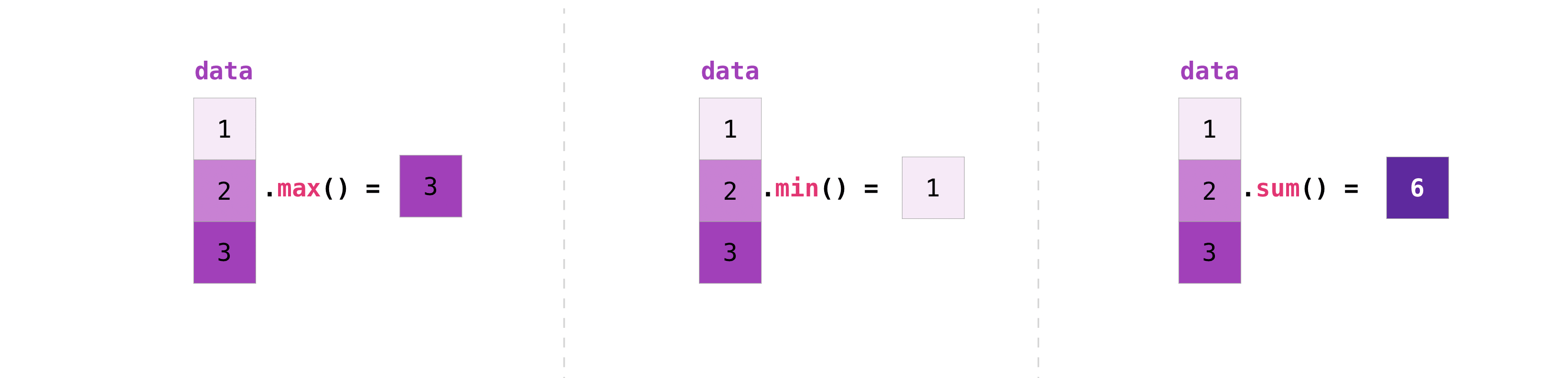
print(f"Maximum: {vector.max()}")
print(f"Index of maximum: {vector.argmax()}")
print(f"Minimum: {vector.min()}")
print(f"Index of minimum: {vector.argmin()}")
print(f"Sum: {vector.sum()}")
print(f"Mean: {vector.mean()}")
print(f"Cumulative sum: {vector.cumsum()}")
vector: [ 9 10 1 2 2 3 3 3 4 5 6 7 8] Maximum: 10 Index of maximum: 1 Minimum: 1 Index of minimum: 2 Sum: 63 Mean: 4.846153846153846 Cumulative sum: [ 9 19 20 22 24 27 30 33 37 42 48 55 63]
print(f"Standard deviation: {vector.std():.3f}")
print(f"Variance: {vector.var():.3f}")
Standard deviation: 2.797 Variance: 7.822
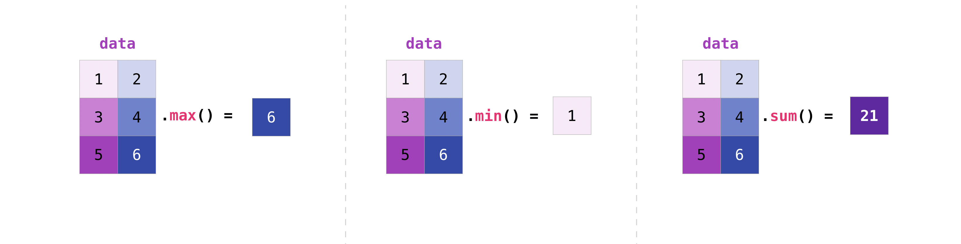
In matrices, axes are defined on which mathematical operations can be performed. By default, operations are performed on all elements of the matrix, but you can specify the axis on which you want to operate.
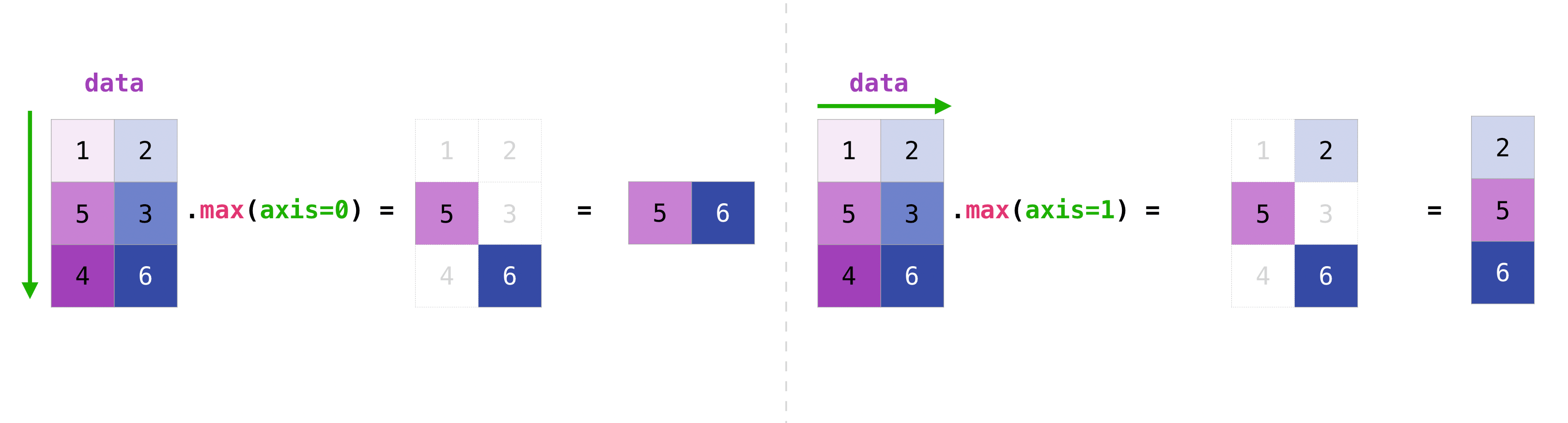
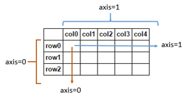
matrix = np.array([[1, 2, 3, 4], [5, 6, 7, 8], [9,10,11,12]])
print(matrix.sum()) # Sum of all elements
print(matrix.sum(axis=0)) # Sum by columns
print(matrix.sum(axis=1)) # Sum by rows
78 [15 18 21 24] [10 26 42]
Operations on matrices
Sorting
print(f"vector before sort:   {vector}")
print("--- Sorting procedurally ---")
# The sort() function receives the vector as an argument and returns it sorted, but does not modify the original vector
sorted_vec = np.sort(vector)
print(f"vector after sort: {vector}")
print(f"sorted:               {sorted_vec}")

print("--- Sorting object-oriented ---")
# The sort() method of the ndarray object modifies the object from which it is called, returns nothing
vector_copy = vector.copy() # copy of the original vector
print(f"vector before sort:   {vector_copy}")
vector_copy.sort()
print(f"sorted vector:        {vector_copy}")
vector before sort: [ 9 10 1 2 2 3 3 3 4 5 6 7 8] --- Sorting procedurally --- vector after sort: [ 9 10 1 2 2 3 3 3 4 5 6 7 8] sorted: [ 1 2 2 3 3 3 4 5 6 7 8 9 10] --- Sorting object-oriented --- vector before sort: [ 9 10 1 2 2 3 3 3 4 5 6 7 8] sorted vector: [ 1 2 2 3 3 3 4 5 6 7 8 9 10]
Unique
# numpy.unique() returns the unique values of a vector
unique_vals, positions = np.unique(vector, return_index=True) # return_index=True returns the indices of unique values
print(f"vector:     {vector}")
print(f"unique:     {unique_vals}")
print(f"indices:    {positions}")
vector: [ 9 10 1 2 2 3 3 3 4 5 6 7 8] unique: [ 1 2 3 4 5 6 7 8 9 10] indices: [ 2 3 5 8 9 10 11 12 0 1]
unique_vals, frequencies = np.unique(vector, return_counts=True) # return_counts=True returns the frequencies of unique values
print(f"vector:      {vector}")
print(f"unique:       {unique_vals}")
print(f"frequencies: {frequencies}")
# If for example we want a dictionary with each value and its frequency, we can use zip:
print(dict(zip(unique_vals, frequencies)))
# zip returns an iterator of tuples combining the elements of the iterables we pass it one by one. In this case, we combine the elements of unique_vals and frequencies, which are two NumPy arrays, so zip returns an iterator of NumPy tuples. When passed to dict, we create a dictionary with the tuples as key-value pairs.
vector: [ 9 10 1 2 2 3 3 3 4 5 6 7 8]
unique: [ 1 2 3 4 5 6 7 8 9 10]
frequencies: [1 2 3 1 1 1 1 1 1 1]
{np.int64(1): np.int64(1), np.int64(2): np.int64(2), np.int64(3): np.int64(3), np.int64(4): np.int64(1), np.int64(5): np.int64(1), np.int64(6): np.int64(1), np.int64(7): np.int64(1), np.int64(8): np.int64(1), np.int64(9): np.int64(1), np.int64(10): np.int64(1)}Flip
print(f"vector:    {vector}")
print(f"flipped: {np.flip(vector)}")
vector: [ 9 10 1 2 2 3 3 3 4 5 6 7 8] flipped: [ 8 7 6 5 4 3 3 3 2 2 1 10 9]